
This blog post explores the idea of using a set of trajectory generation equations in conjunction with a neural network for quadruped locomotion. We will discuss the advantages of this approach and how it compares to directly using a neural network to generate joint angle deltas.
My implementation is inspired by the method presented in the paper Policies Modulating Trajectory Generators et al. Atil Iscen, with a few modifications.
Note: Detailed results and video clips can be found in the Results section below.
Why Use a Trajectory Generator?
You might wonder why this method is necessary when direct neural network-based control has already shown promising results, as demonstrated in our previous post on blind locomotion using proprioception. The key advantage of using a trajectory generator (TG) is that it produces cleaner gaits with minimal reward function tuning. Since the gait is defined by a system of equations, the neural network is relieved from learning the complexities of generating a stable gait. Instead, the network focuses on modulation and stabilization, leading to more efficient learning and better overall performance.
Paper Overview
Before diving into our custom implementation, let’s examine the approach used in the original paper.
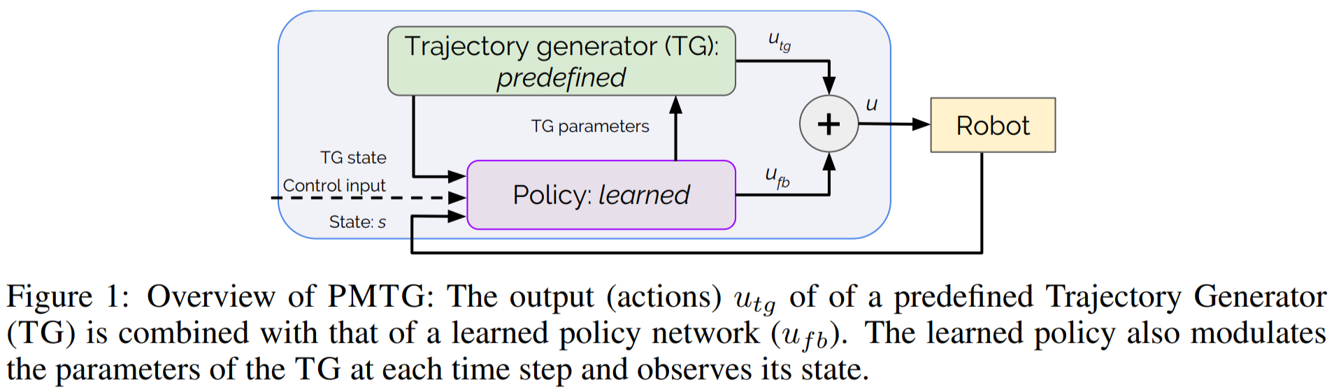
As illustrated in the figure below, the trajectory generator is indirectly controlled by a subset of the policy’s output (TG Parameters). These parameters are set based on the TG state along with other inputs to the policy. The final joint position command sent to the robot is the sum of the TG’s output and the policy’s modulation.
In an ideal scenario, even if the policy outputs zero joint modifications, the trajectory generator should still produce a trotting motion, allowing the robot to trot in place. The policy’s primary task is to stabilize this motion and modulate it as needed to achieve locomotion by adjusting the phase, height, or stride length of the legs.
To understand the implementation in more detail, let’s take a look at the parameters that the policy sets.
From the paper:
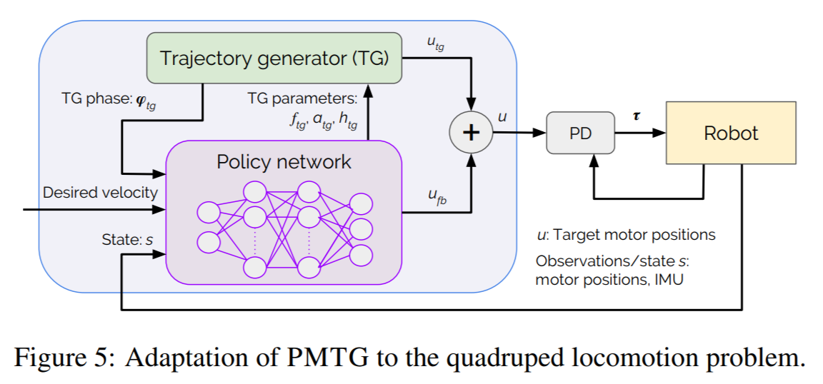
The detailed architecture adapted to quadruped locomotion is shown in Fig. 5. At every timestep, the policy receives observations (s), desired velocity (v, control input) and the phase (φ) of the trajectory generator. It computes 3 parameters for the TG (frequency f, amplitude a and walking height h) and 8 actions for the legs of the robot ($u_{fb}$) that will directly be added to the TG’s calculated leg positions ($u_{tg}$). The sum of these actions is used as desired motor positions, which are tracked by Proportional-Derivative controllers. Since the policy dictates the frequency at each time step, it dictates the step-size that will be added to TG’s phase. This eventually allows the policy to warp time and use the TG in a time-independent fashion.
Custom Implementation
The custom implementation is strongly inspired by the above paper and method but has some crucial changes that helped with a smoother implementation.
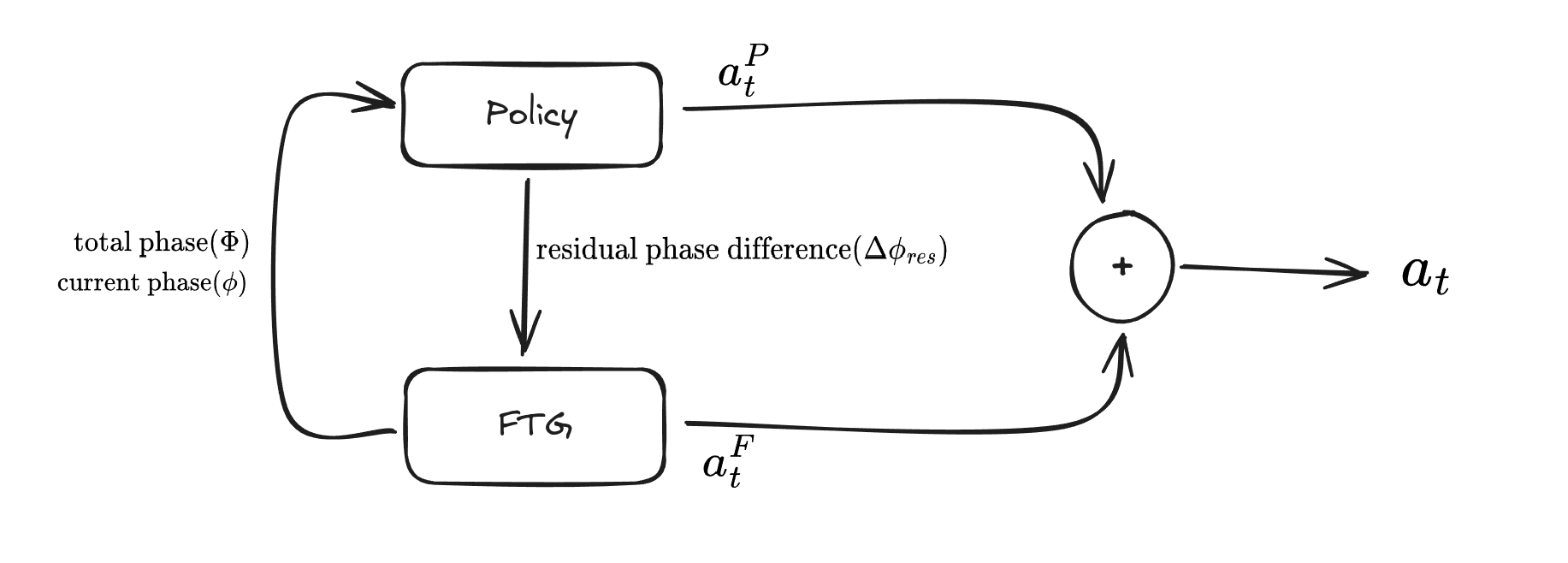
The most important changes are to the inputs to the FTG from the policy consisting of only the residual phase differences and the policy input consisting of total phase and current phases for each legs.
Here is a detailed breakdown to further explain things: The policy output can be broken down into two components: joint actions ${(a_t^P)}$ and residual phase difference $(\Delta\phi_{res})$
The height of each leg as a function of the total phase$(\Phi)$ of the leg $h(\Phi)$ in the FTG can be expressed using the following formula
\[\begin{aligned} h(\Phi) = \begin{cases} h_{\max} \left(-2\left(\dfrac{2}{\pi}\Phi\right)^3 + 3\left(\dfrac{2}{\pi}\Phi\right)^2\right), & \text{if } 0 \leq \Phi \leq \frac{\pi}{2}, \\ h_{\max} \left(2\left(\dfrac{2}{\pi}\Phi - 1\right)^3 - 3\left(\dfrac{2}{\pi}\Phi - 1\right)^2 + 1\right), & \text{if } \frac{\pi}{2} < \Phi \leq \pi, \\ 0, & \text{if } \pi < \Phi < 2\pi. \end{cases} \end{aligned}\]The total phase of the leg $(\Phi)$ is computed using the following formula:
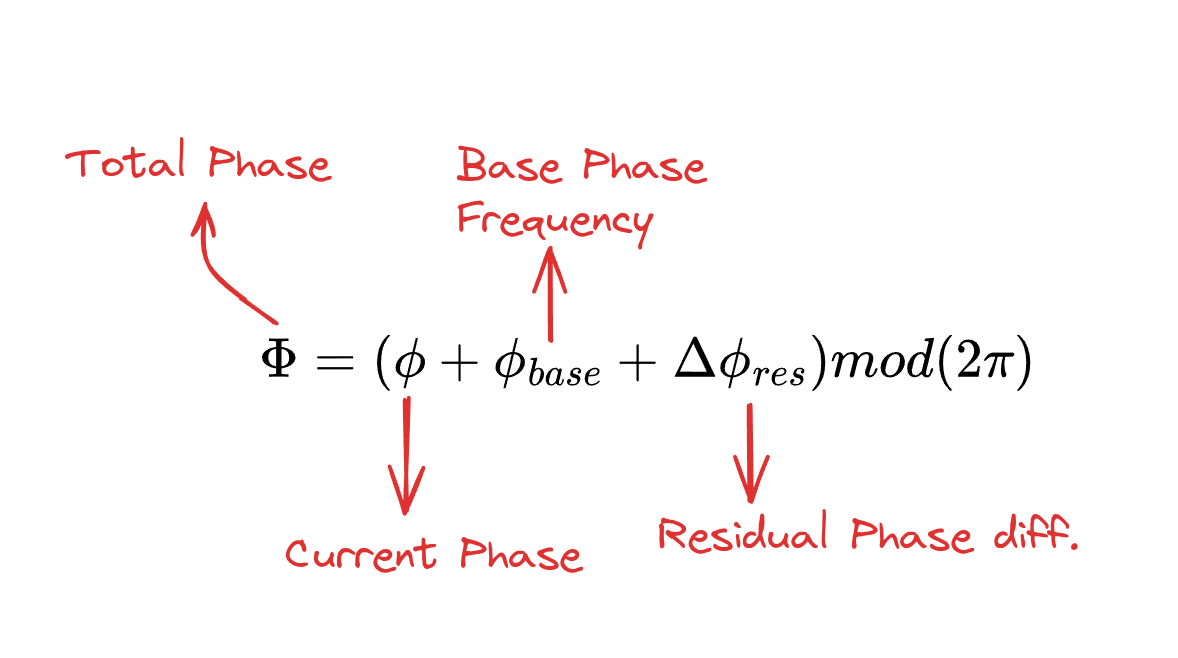
In the above equation, $\phi$ is the current phase that is incremented each time step as follows $\phi_{t+1} = ( \phi_t + \Delta\phi) \text{ mod}(2\pi)$ where $\Delta\phi$ is a constant like 0.2
In the above equation, $\phi_{base}$ is used to encode a gait prior by setting in the phase difference between different legs in the robot, its value is usually like
\[\phi_{base} = \begin{cases} [0, \pi, \pi, 0], & \text{if walk}\\ [\pi, \pi, 0, 0], & \text{if gallop}\\ [0, 0, 0, 0], & \text{if stand}\\ \end{cases}\]And finally $\Delta\phi_{res}$ is the residual phase difference that can be set by the policy as part of its output to make adjustments to the total phase of each leg.
The height of each foot is now used to compute the joint angles for each leg using Inverse Kinematics as follows:
For the First Joint Angle $(q_1)$
\[L = \sqrt{p_y^2 + p_z^2 - l_1^2}\] \[q_1 = \arctan\!\left(\frac{p_z\, l_1 + p_y\, L}{p_y\, l_1 - p_z\, L}\right)\]For the Third Joint Angle $(q_3)$
\[\text{temp} = \frac{b_{3z}^2 + b_{4z}^2 - b^2}{2\,\left|b_{3z}\, b_{4z}\right|}\] \[q_3 = -\Bigl(\pi - \arccos\bigl(\text{temp}\bigr)\Bigr)\]For the Second Joint Angle $(q_2)$
\[a_1 = p_y \sin(q_1) - p_z \cos(q_1)\] \[a_2 = p_x\] \[m_1 = b_{4z} \sin(q_3)\] \[m_2 = b_{3z} + b_{4z} \cos(q_3)\] \[q_2 = \arctan\!\left(\frac{m_1\, a_1 + m_2\, a_2}{m_1\, a_2 - m_2\, a_1}\right)\]Body Orientation Adjustment is done using the following transformations
Roll rotation matrix (for roll angle $\alpha$)
\[R\_{\text{roll}} = \begin{pmatrix} 1 & 0 & 0 \\ 0 & \cos\alpha & -\sin\alpha \\ 0 & \sin\alpha & \cos\alpha \end{pmatrix}\]Pitch rotation matrix (for pitch angle $\beta$)
\[R\_{\text{pitch}} = \begin{pmatrix} \cos\beta & 0 & -\sin\beta \\ 0 & 1 & 0 \\ \sin\beta & 0 & \cos\beta \end{pmatrix}\]Combined rotation to adjust the foot position vector $\mathbf{p}$
\[\mathbf{p}_{\text{adjusted}} = R_{\text{pitch}} \, R\_{\text{roll}} \, \mathbf{p}\]For your reference here is what each of these variables mean:
$p_x,p_y,p_z$ are the Cartesian coordinates of the foot’s target position in the robot’s coordinate system.
- $p_x$ is the position along the forward-backward direction.
- $p_y$ is the lateral position (side-to-side).
- $p_z$ is the vertical position (height).
$l_1,l_2,l_3$ are the lengths of the segments (links) in the leg.
- $l_1$ corresponds to the distance from the hip to the first joint.
- $l_2$ corresponds to the second segment (e.g., thigh length).
- $l_3$ corresponds to the third segment (e.g., shank length).
$L$ is an auxiliary variable defined as:
\[L =\sqrt{p_y^2+p_z^2-l_1^2}\]It helps in computing the first joint angle by combining the lateral and vertical components.
- $q_1$ The first joint angle, computed using the positions $p_x$ and $p_y$ along with the link length $l_1$. It primarily handles the orientation of the leg in the vertical plane.
- $b_{3z}$ and $b_{4z}$ These represent the effective lengths (or offsets) associated with the second and third segments of the leg. In many implementations, they are set as $-l_2$ and $-l_3$
The final actions $a_t$ that are passed on to the PD controller can now be computed using the following equation:
\[a_t = \alpha .a_t^P + a_t^F\]Where $\alpha$ is the weight given to the joint actions from the policy.
Results
Here is a compilation video of the FTG based locomotion policy being implemented, this was just a quick test of the method for a richer and complete implementation have a look at my post on Locomotion with Weighted Belief in Exteroception where FTG is reused.