
A project on achieving realtime-orthomosaic SLAM for aerial navigation using a single downwards facing camera in outdoor GPS denied environments.
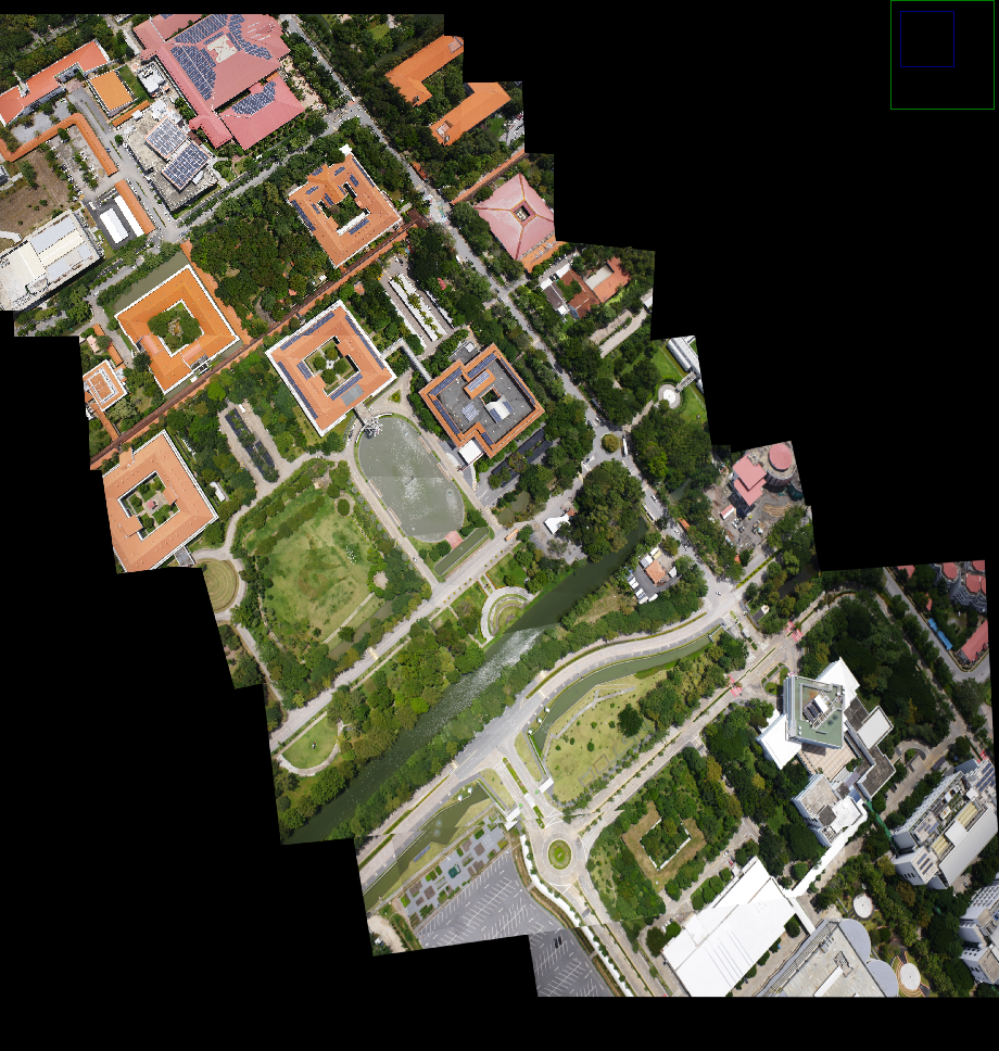
Results
Introduction
To carry out drone-based aerial surveying for generating orthomosaic maps on the fly, this project explores the image processing stack required to achieve the same using the most economical hardware and software footprint. The project explores corner and blob-based feature extraction techniques followed by brute force and KNN based feature matching methods which are later used to generate a homography matrix for stitching images passed through a cascaded image mixer to generate orthomosaic maps of a given dataset.

Feature Detection & Extraction
While there is no universally accepted definition of “Feature” for a given image, it is often regarded as the information that is unique for the given image and thus helps us mathematically associate the image with its unique data properties.
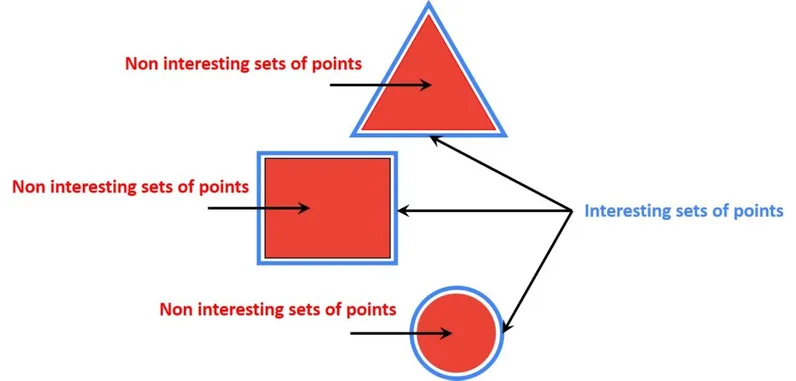
Image Features are small patches of unique raw data that can be potentially used to differentiate the given image from any other image, therefore, helping in tracking the similarity between given images. Image Features can be broken down into two major components:
1) Keypoints 2) Descriptor
They are explained in the subsequent sections.
Keypoints
Keypoints contain 2D patch data like position, scale, convergence area, and other properties of the local patch. Which we define as a distinctive point in an input image that is invariant to rotation, scale, and distortion. In practice, the key points are not perfectly invariant but they are a good approximation. [1]
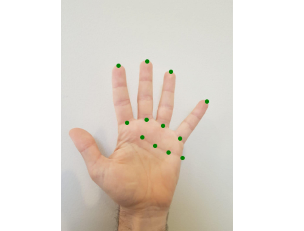 Example: Keypoints of a human hand.
Descriptors & Detectors
A feature detector is an algorithm that takes an image and produces the positions (pixel coordinates) of important regions in the picture. A corner detector is an illustration of this, since it outputs the positions of corners in your picture but does not provide any other information about the features discovered.
A feature descriptor is an algorithm that takes an image and generates feature descriptors/feature vectors from it.[2] Feature descriptors encapsulate important information into a sequence of numbers and serve as a numerical “fingerprint” that may be used to distinguish one feature from another. They highlight various keypoint properties in vector format (constant length). It might be their intensity in the direction of their most pronounced orientation, for example. It is giving a numerical description of the area of the image to which the keypoint is referenced.
Important properties of descriptors
-
they should be independent of keypoint position If the same keypoint is extracted at different positions (e.g. because of translation) the descriptor should be the same. [3]
- they should be robust against image transformations Variations in contrast (for example, a photograph of the same location on a bright and overcast day) and changes in perspective are two examples (image of a building from center-right and center-left, we would still like to recognize it as the same building). Of all, no description is absolutely impervious to all modifications (nor against any single one if it is strong, e.g. big change in perspective). Different descriptors are meant to be resistant against various transformations, which are sometimes incompatible with the speed at which they are calculated. [3]
- they should be scale independent The scale should be considered in the descriptions. If the “prominent” component of one key point is a vertical line of 10px (within a circular area with a radius of 8px), and the prominent part of another is a vertical line of 5px (inside a circular area with a radius of 4px), the descriptions for both key points should be identical. [3]
Available Methods
Shi-Tomasi Corner Detector
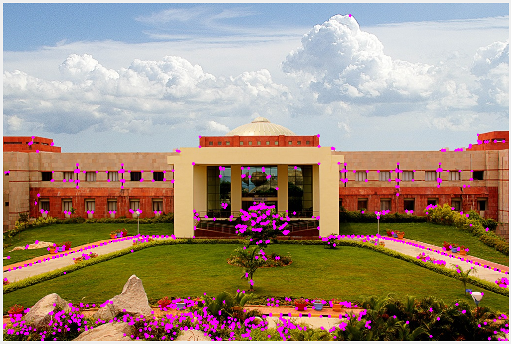
Example: Using Good Features to Track to detect keypoints
The Shi-Tomasi Corner Detector is a modified version of the Harris Corner Detector with the primary change being in the way in which the score “R” is calculated making it more efficient than the standard Harris Corner Detector.
Corners are considered as areas in photographs where a little alteration in position, results in a significant change in intensity in both the horizontal (X) and vertical (Y) axes.
The Pseudocode for Shi-Tomasi Corner Detector:
- Determine windows of small image patches that produce very large variations in intensity when moved in both X and Y directions (i.e. gradients).[4]
- Compute score R for each such window. 3, Apply a threshold to select and retrieve important corner points.
Python Implementation of Shi-Tomasi Corner Detector:
1
2
3
4
5
6
7
8
9
10
11
12
13
import cv2
import numpy as np
img_1 = cv2.imread('images/admin_block.jpg')
gray = cv2.cvtColor(img_1, cv2.COLOR_BGR2GRAY)
cv2.namedWindow("output", cv2.WINDOW_NORMAL)
corners = cv2.goodFeaturesToTrack(gray, 1000, 0.01, 1)
corners = np.int0(corners)
for i in corners:
x, y = i.ravel()
cv2.circle(img_1, (x, y), 3, (255, 0, 255), -1)
cv2.imshow("output", img_1)
cv2.waitKey(0)
cv2.destroyAllWindows()
OpenCV has implemented a function cv2.goodFeaturesToTrack() the parameters for this function are:
- image - Input 8-bit or floating-point 32-bit, single-channel image
- maxCorners - Maximum number of corners to detect. If the number of corners on an image is higher than the number of maxCorners the most pronounced corners are selected.
- qualityLevel - Parameter characterizing the minimal accepted quality of image corners. All corners below the quality level are rejected. The parameter value is multiplied by the best corner quality measure, which is the minimal eigenvalue of the Harris function response.[5]
- minDistance - minimal Euclidean distance between corners
Scale Invariant Feature Transform (SIFT)
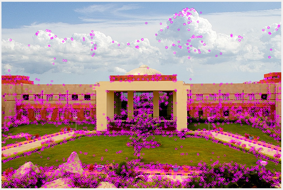 Example: Using SIFT to detect keypoints
SIFT, which stands for Scale-Invariant Feature Transform, was introduced in 2004 by D.Lowe of the University of British Columbia. This algorithm is robust against image scale variations and rotation invariances.
The Pseudocode for SIFT:
- Scale-space peak selection: Potential location for finding features.
- Keypoint Localization: Accurately locating the feature keypoints.
- Orientation Assignment: Assigning orientation to keypoints.
- Keypoint descriptor: Describing the keypoints as a high dimensional vector.
- Keypoint Matching
The Python Implementation for SIFT:
1
2
3
4
5
6
7
8
9
10
import cv2
import numpy as np
img = cv2.imread'(images/admin_block.jpg')
img_gray = cv2.cvtColor(img, cv2.COLOR_BRG2GRAY)
cv2.namedWindow("output", cv2.WINDOW_NORMAL)
sift = cv2.SIFT_create()
kypoints = sift.detect(img_gray, None)
cv2.imshow("output", cv2.drawKeypoints(img, keypoints, None, (255, 0, 255)))
cv2.waitKey(0)
cv2.destroyAllWindows()
Parameters for SIFT:
- nfeatures - The number of best features to retain. The features are ranked by their scores (measured in SIFT algorithm as the local contrast)
- nOctaveLayers - The number of layers in each octave. 3 is the value used in D. Lowe’s paper. The number of octaves is computed automatically from the image resolution.
- contrastThreshold - The contrast threshold is used to filter out weak features in semi-uniform (low-contrast) regions. The larger the threshold, the fewer features are produced by the detector.
Speeded Up Robust Features (SURF)
The SURF (Speeded Up Robust Features) technique is a quick and robust approach for local, similarity invariant picture representation and comparison. The SURF approach’s prominent feature is its quick computing of operators using box filters, which enables real-time applications such as tracking and object identification.
The Pseducode for SURF:
- Feature Extraction
- Hessian matrix-based interest points
- Scale-space representation
- Feature Description
- Orientation Assignment
- Descriptor Components
The python implementation of SURF:
1
2
3
4
5
6
7
8
9
10
import cv2
import numpy as np
img = cv2.imread'(images/admin_block.jpg')
img_gray = cv2.cvtColor(img, cv2.COLOR_BRG2GRAY)
cv2.namedWindow("output", cv2.WINDOW_NORMAL)
surf = cv2.xfeatures2d.SURF_create()
kypoints = surf.detect(img_gray, None)
cv2.imshow("output", cv2.drawKeypoints(img, keypoints, None, (255, 0, 255)))
cv2.waitKey(0)
cv2.destroyAllWindows()
public static SURF create(double hessianThreshold, int nOctaves, int nOctaveLayers, boolean extended, boolean upright)
Parameters for SURF:
- hessianThreshold - Threshold for hessian keypoint detector used in SURF.
- nOctaves - Number of pyramid octaves the keypoint detector will use.
- nOctaveLayers - Number of octave layers within each octave.
- extended - Extended descriptor flag (true - use extended 128-element descriptors; false - use 64-element descriptors).
- upright - Up-right or rotated features flag (true - do not compute the orientation of features; false - compute orientation).
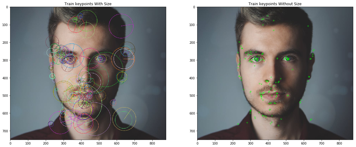
Oriented FAST and Rotated BRIEF (ORB)
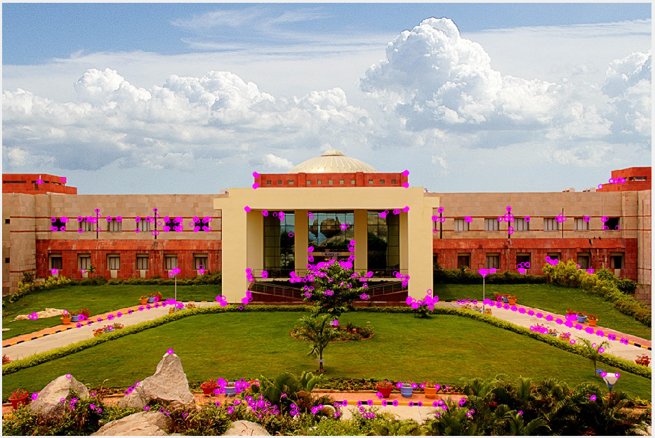
Example: Using ORB to detect keypoints
ORB is a combination of the FAST keypoint detector and the BRIEF descriptor, with some additional characteristics to boost performance. FAST stands for Features from Accelerated Segment Test, and it is used to find features in a picture. It also employs a pyramid to generate multiscale features.[2] It no longer computes the orientation and descriptors for the features, which is where BRIEF is used.
ORB employs BRIEF descriptors, although the BRIEF performs badly when rotated. So what ORB does is rotate the BRIEF according to the keypoint orientation. The rotation matrix of the patch is calculated using the patch’s orientation, and the BRIEF is rotated to obtain the rotated version.
The Pseudocode for ORB:[7]
- Take the query image and convert it to grayscale.
- Now Initialize the ORB detector and detect the keypoints in query image and scene.
- Compute the descriptors belonging to both images.
- Match the keypoints using Brute Force Matcher.
- Show the matched images.
The Python implementation of ORB:
1
2
3
4
5
6
7
8
9
10
import cv2
import numpy as np
img = cv2.imread'(images/admin_block.jpg')
img_gray = cv2.cvtColor(img, cv2.COLOR_BRG2GRAY)
cv2.namedWindow("output", cv2.WINDOW_NORMAL)
orb = cv2.ORB_create(nfeatures = 1000)
kypoints_orb, descriptors = orb.detectAndCompute(img_1, None)
cv2.imshow("output", cv2.drawKeypoints(img_1, keypoints_orb, None, (255, 0, 255)))
cv2.waitKey(0)
cv2.destroyAllWindows()
Conclusion
- One of the notable drawbacks of the Shi-Tomasi Corner Detector is the fact that it is not scale-invariant.
- ORB is a more efficient feature extraction approach than SIFT or SURF in terms of computing cost, matching performance, and, most importantly, patents.
- SIFT and SURF are patented, and you are required to pay for their use. However, ORB is not patented.
Feature Matching
Available Methods
Brute Force Matcher
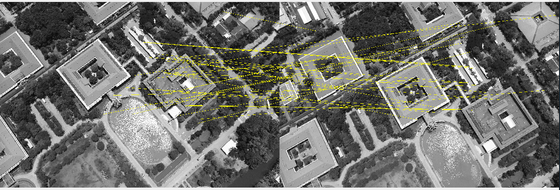
The Brute Force Matcher is used to compare the characteristics of the first image to those of another image.
It takes one of the first picture’s descriptors and matches it to all of the second image’s descriptors, then moves on to the second descriptor of the first image and matches it to all of the second image’s descriptors, and so on.
Homography & Transformation
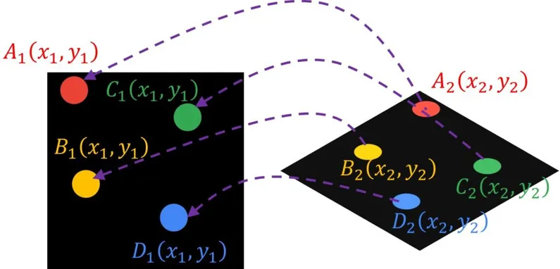
A homography connects any two photographs of the same scene. It is a transformation that transfers the points in one picture to the points in the other. The two pictures can be captured by rotating the camera along its optical axis or by laying them on the same surface in space.
The essence of the homography is the simple 3×3 matrix called the homography matrix.
This matrix may be applied to any spot in the picture. For example, in the first image, if we choose a position A(x1,y1), we may use a homography matrix to translate this point A to the matching point B(x2,y2) in the second image.
The python implementation of finding homography matrix:
1
2
3
4
5
6
7
8
9
10
11
12
13
14
15
16
17
18
19
20
21
22
23
def wrap_images(self, image1, image2, H):
    rows1, cols1 = image1.shape[:2]
    rows2, cols2 = image2.shape[:2]
    H = H
    list_of_points_1 = np.float32(
        [[0, 0], [0, rows1], [cols1, rows1], [cols1, 0]]).reshape(-1, 1, 2)
    temp_points = np.float32(
        [[0, 0], [0, rows2], [cols2, rows2], [cols2, 0]]).reshape(-1, 1, 2)
    # When we have established a homography we need to warp perspective
    # Change field of view
    list_of_points_2 = cv2.perspectiveTransform(temp_points, H)
    list_of_points = np.concatenate(
        (list_of_points_1, list_of_points_2), axis=0)
    [x_min, y_min] = np.int32(list_of_points.min(axis=0).ravel() - 0.5)
    [x_max, y_max] = np.int32(list_of_points.max(axis=0).ravel() + 0.5)
    translation_dist = [-x_min, -y_min]
    H_translation = np.array([[1, 0, translation_dist[0]], [
        0, 1, translation_dist[1]], [0, 0, 1]])
    output_img = cv2.warpPerspective(
        image2, H_translation.dot(H), (x_max-x_min, y_max-y_min))
    output_img[translation_dist[1]:rows1+translation_dist[1],
        translation_dist[0]:cols1+translation_dist[0]] = image1
    return output_img
It is important to realize that feature matching does not always provide perfect matches. As a result, the Random Sample Consensus (RANSAC) process is used as a parameter in the cv2.findHomography() method, making the algorithm robust to outliers. We can get reliable results using this strategy even if we have a large percentage of bad matches.
Python Implementation of RANSAC:
1
2
3
4
5
6
7
8
9
10
11
12
13
14
15
16
17
18
19
# Set minimum match condition
MIN_MATCH_COUNT = 2
if len(good) > MIN_MATCH_COUNT:
    # Convert keypoints to an argument for findHomography
    src_pts = np.float32(
    [keypoints1[m.queryIdx].pt for m in good]).reshape(-1, 1, 2)
    dst_pts = np.float32(
    [keypoints2[m.trainIdx].pt for m in good]).reshape(-1, 1, 2)
    # Establish a homography
    M, _ = cv2.findHomography(src_pts, dst_pts, cv2.RANSAC, 5.0)
    result = self.wrap_images(image2, image1, M)
    # cv2.imwrite('test4.jpg',result)
    # cv2.imshow("output_image",result)
    # cv2.waitKey(0)
    # cv2.destroyAllWindows()
    return result
else:
    print("Error")
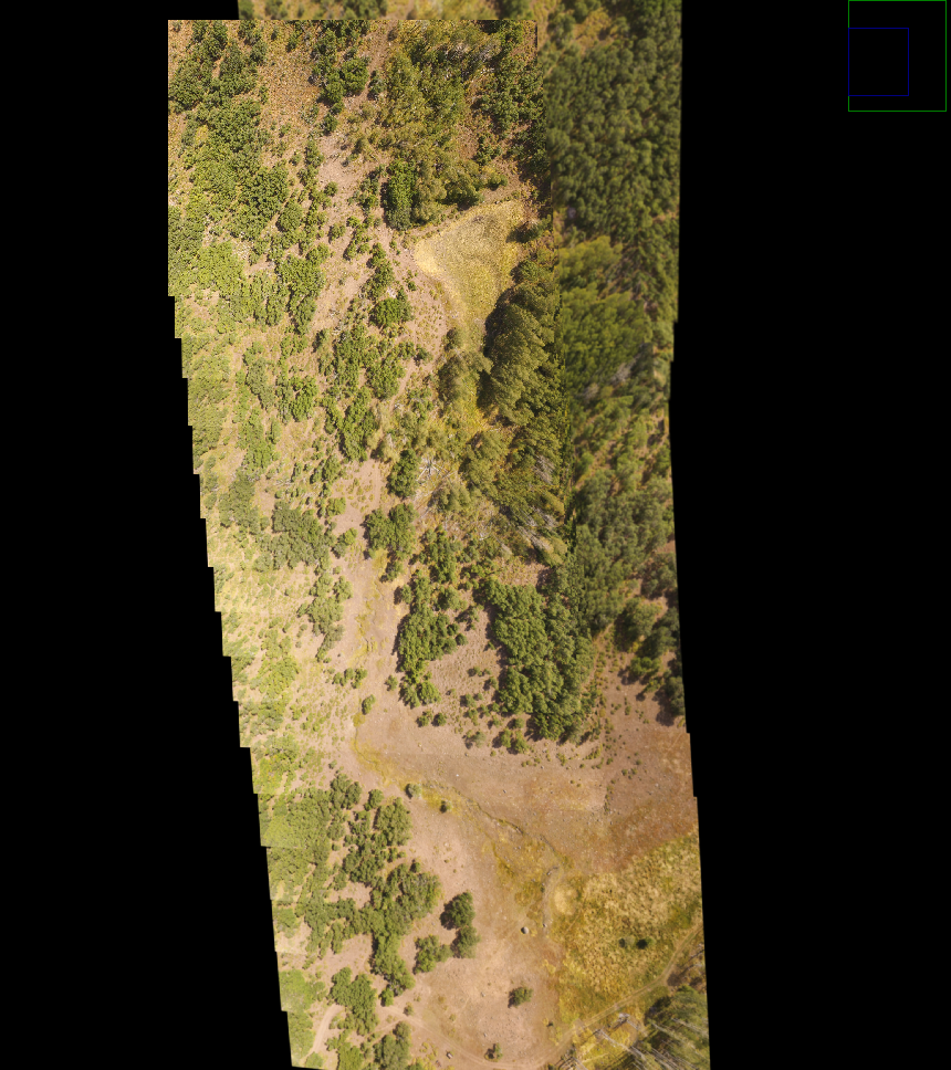
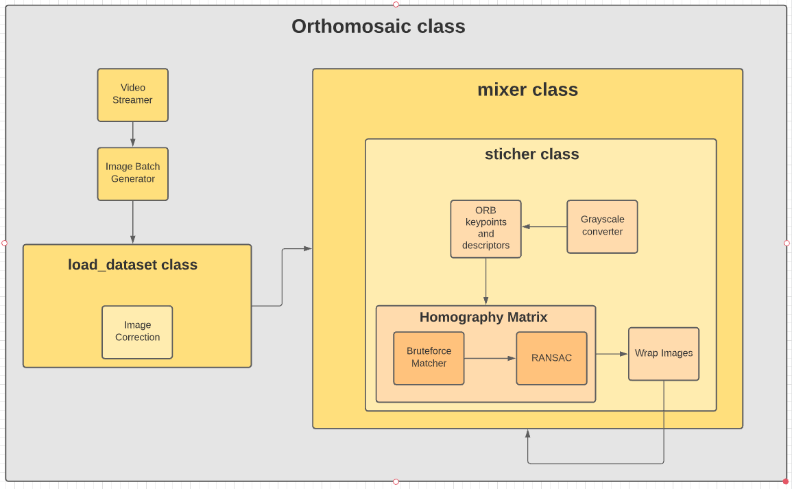
Image Processing Pipeline
Dataset
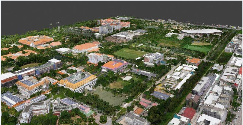
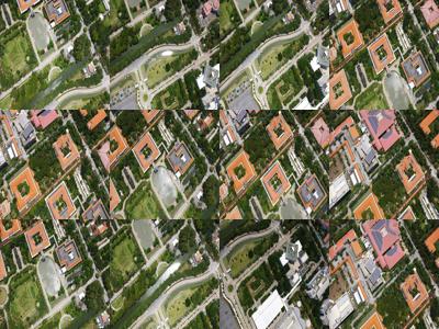
Urban Area
This dataset of the Thammasat University campus in Bangkok, Thailand was collected by a senseFly eBee X drone carrying a senseFly Aeria X photogrammetry camera.
Technical Details |Feature|Value| |–|–| Ground resolution|6 cm (3.36 in)/px Coverage|2.1 sq. km (0.77 sq. mi) Flight height|285 m (935 ft) Number of images|443
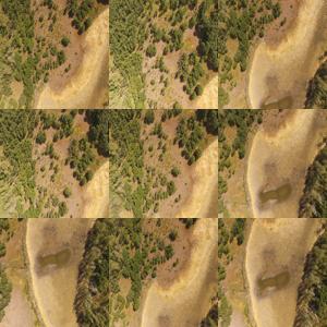
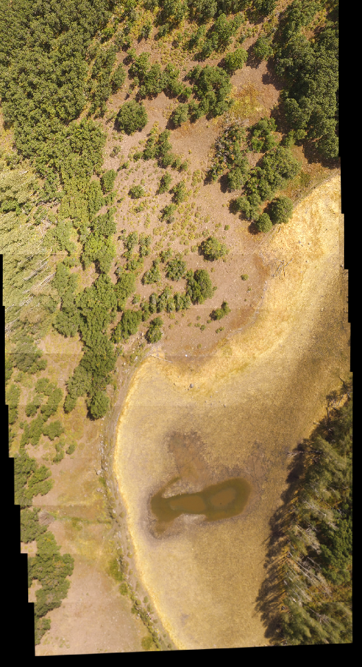
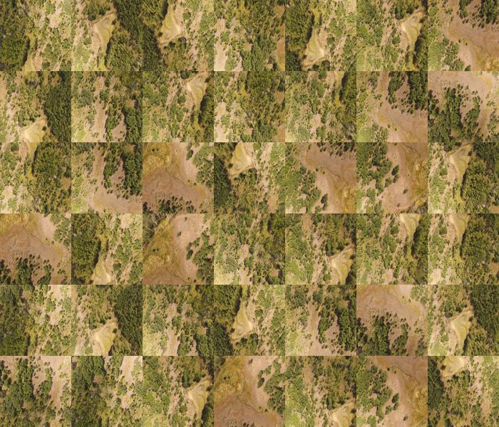
Forest Area
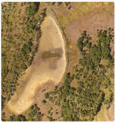
DroneMapper flew Greg 1 and 2 reservoirs on September 16th, 2019 using their Phantom 3 Advanced drone to collect imagery for precision digital elevation model (DEM) and orthomosaic generation of the site. GCP was surveyed with a Trimble 5800 and used during the image processing. Approximately 189 images were collected and processed via photogrammetry to yield the DEM, orthomosaic, and capacity report.[8]
| Feature | Value |
|---|---|
| Ground resolution | 6 cm (3.36 in)/px |
| Coverage | 2.1 sq. km (0.77 sq. mi) |
| Flight height | 285 m (935 ft) |
| Number of images | 189 |
Future Work
Use it for realtime localization in Gazebo.