This post is part of the Deep Reinforcement Learning Blog Series. For a detailed introduction about the series, the curicullum, sources and references used, please check Part 0 - Getting Started.
Structure of the blog
- Part 0 - Getting Started
- Part 1 - Multi-Arm Bandits
- Part 2 - Finite MDP | Prerequisites: python, gymnasium, numpy
- Part 3 - Dynamic Programming | Prerequisites: python, gymnasium, numpy
- Part 4 - Monte Carlo, Temporal Difference & Bootstrapping Methods | Prerequisites: Python, gymnasium, numpy
- Part 5 - Deep SARSA and Q-Learning | Prerequisites: python, gymnasium, numpy, torch
- Part 6 - REINFORCE, AC, DDPG, TD3, SAC
- Part 7 - A2C, PPO, TRPO, GAE, A3C
- TBA (HER, PER, Distillation)
Monte Carlo Methods
MC methods improvise over DP methods as they can be used in cases where we do not have a model of the environment. They do this by learning from episodes of experience. Therefore one caviat of MC methods is that they do not work on continous MDPs and learn only from complete episodes (Episodes must terminate).
Monte Carlo Prediction
We begin by considering Monte Carlo methods for learning the state-value function for a given policy. Recall that the value of a state is the expected return—expected cumulative future discounted reward—starting from that state. An obvious way to estimate it from experience, then, is simply to average the returns observed after visits to that state. As more returns are observed, the average should converge to the expected value. This idea underlies all Monte Carlo methods.
On-Policy MC Prediction
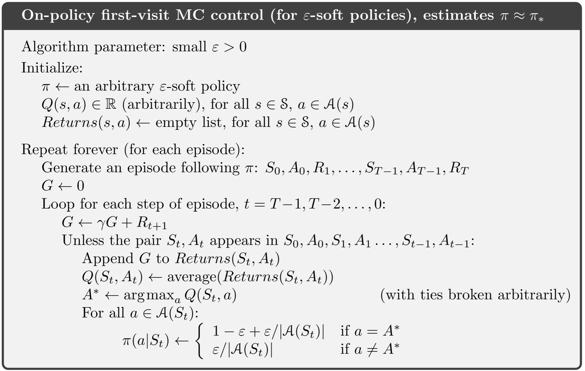
We have a small variation in the fact that we can consider each state only the first time it has been visited while estimating the mean return or we can account for multiple visits to the same state(if any) and the follwoing pseudocodes illustrate both the variations
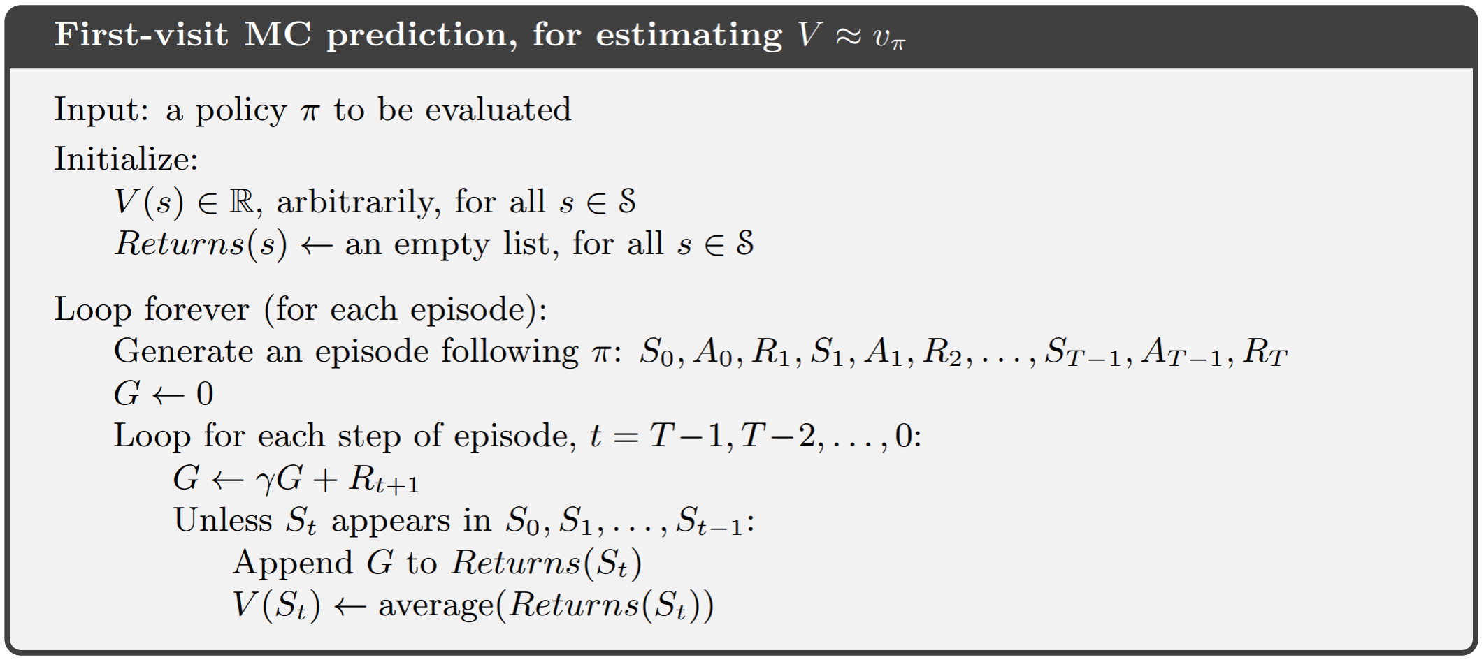
The every-visit version can be implemented by removing the “Unless $S_t$ appears in $S_0$, $S_1$, … $S_{t-1}$” line.
Incremental Updates
A more computationally efficient method would be to calculate the mean incrementally as follows:
- Update $V(s)$ incrementally after episode $S_1,A_1,R_2,….,S_T$
- For each state $S_t$ with return $G_t$
For non-stationary problems, it can be useful to track a running mean (forgets old epiosdes and gives more weight to recent experiences).
\[V(S_t) \leftarrow V(S_t) + \alpha(G_t-V(S_t))\]Off-Policy MC Prediction
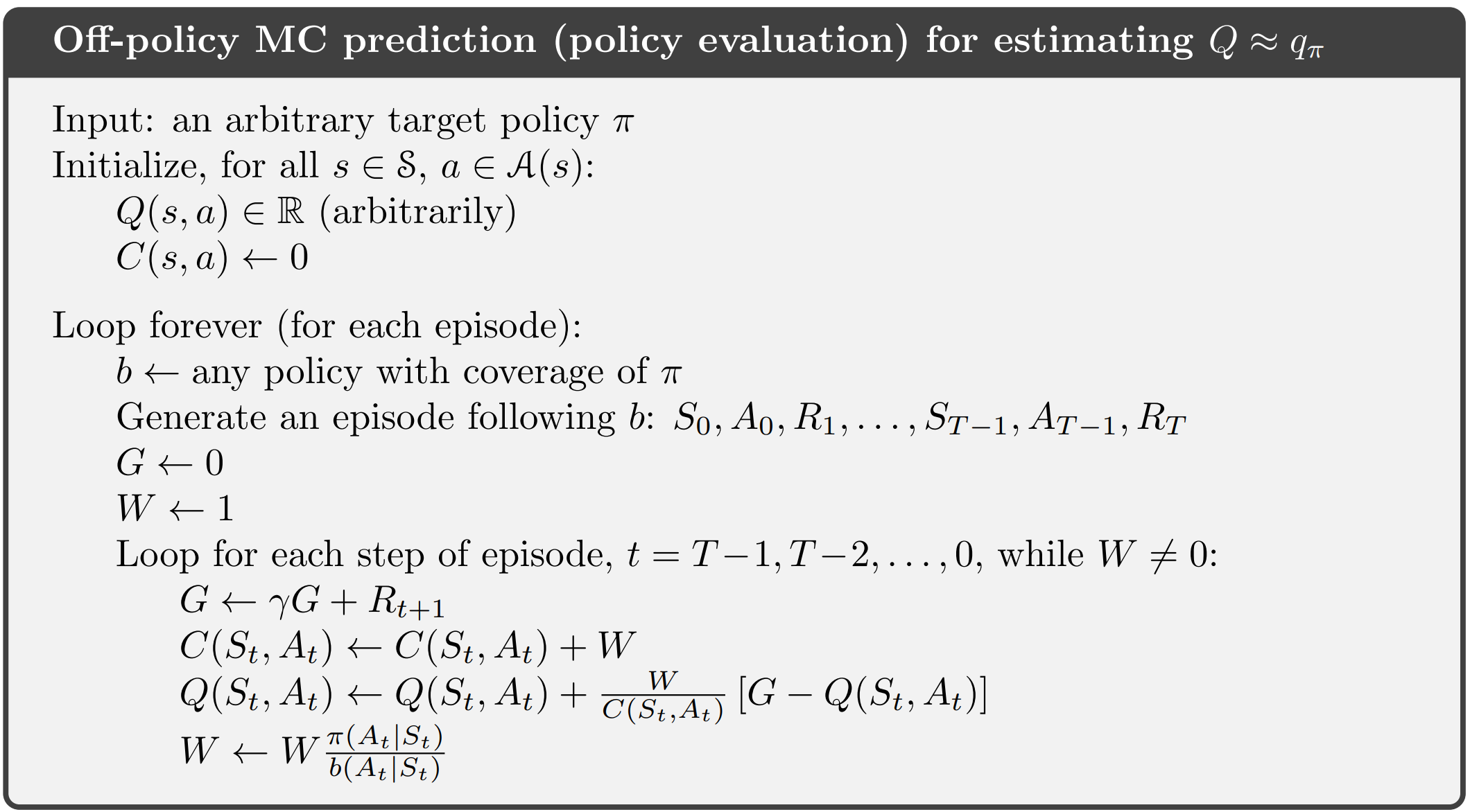
Almost all off-policy methods utilize importance sampling, a general technique for estimating expected values under one distribution given samples from another. We apply importance sampling to off-policy learning by weighting returns according to the relative probability of their trajectories occurring under the target and behavior policies, called the importance-sampling ratio. Off-Policy Monte Carlo Prediction can be implemented via two variations of importance sampling which are discussed below.
Ordinary Importance Sampling
For evaluating a terget policy $\pi(a|s)$ to compute $v_\pi(s)$ or $q_\pi(s,a)$ while following a behaviour policy $\mu(a|s)$.
Given, \(\{S_1,A_1,R_2,...,S_T\} \sim \mu\)
We can weight returns $G_t$ according to similarity between the two policies. By multiplying the importance sampling corrections along the whole episode we get:
\[G_t^{\pi/\mu} = \dfrac{\pi(A_t|S_t)\pi(A_{t+1}|S_{t+1})...\pi(A_{T}|S_{T})}{\mu(A_{t}|S_{t})\mu(A_{t+1}|S_{t+1})...\mu(A_{T}|S_{T})}G_t\]We can then update the state value towards the corrected return like this
\[V(S_t) \leftarrow V(S_t) + \alpha(G_t^{\pi/\mu}-V(S_t))\]Note that we cannot use this if $\mu$ is zero when $\pi$ is non-zero, also that importance sampling can increase variance.
Weighted Importance Sampling
 The derivation of the Weighted Importance Sampling equations has been left-out for the time being.
Ordinary importance sampling is unbiased whereas weighted importance sampling is biased (though the bias converges asymptotically to zero). On the other hand, the variance of ordinary importance sampling is in general unbounded because the variance of the ratios can be unbounded, whereas in the weighted estimator the largest weight on any single return is one. In fact, assuming bounded returns, the variance of the weighted importance-sampling estimator converges to zero even if the variance of the ratios themselves is infinite (Precup, Sutton, and Dasgupta 2001). In practice, the weighted estimator usually has dramatically lower variance and is strongly preferred.
Monte Carlo Control
While it might seem straight forward to implement MC Methods in GPI by plugging MC Prediction for policy evaluation and using greedy policy improvement to complete the cycle, there is one key problem that needs to be addressed.
Greedy policy improvement over $V(s)$ requires knowledge about the MDP \(\pi'(s) = \mathtt{argmax}_{a\in A} r(a|s) + p(s'|s,a)V(s')\)
To remain model free we can instead switch to action value functions which will not require prior details about the MDP
\[\pi'(s) = \mathtt{argmax}_{a\in A} Q(s,a)\]While this solves the issue of knowing the model MDP, we now have a deterministic policy and we will never be able to collect experiences of alternative actions and therefore might miss out on exploration altogether.
This can be solved in the following ways:
-
Exploring Starts: Every state-action pair has a non-zero probability of being selected as the starting pair, this ensures sufficient exploration but in reality, this might not always be possible.
-
$\epsilon-$ soft policies: A small probability to explore every time an action is to be choosen.
-
Off-Policy: Use a different policy to collect experience than the one target policy being improved.
On-Policy MC Control
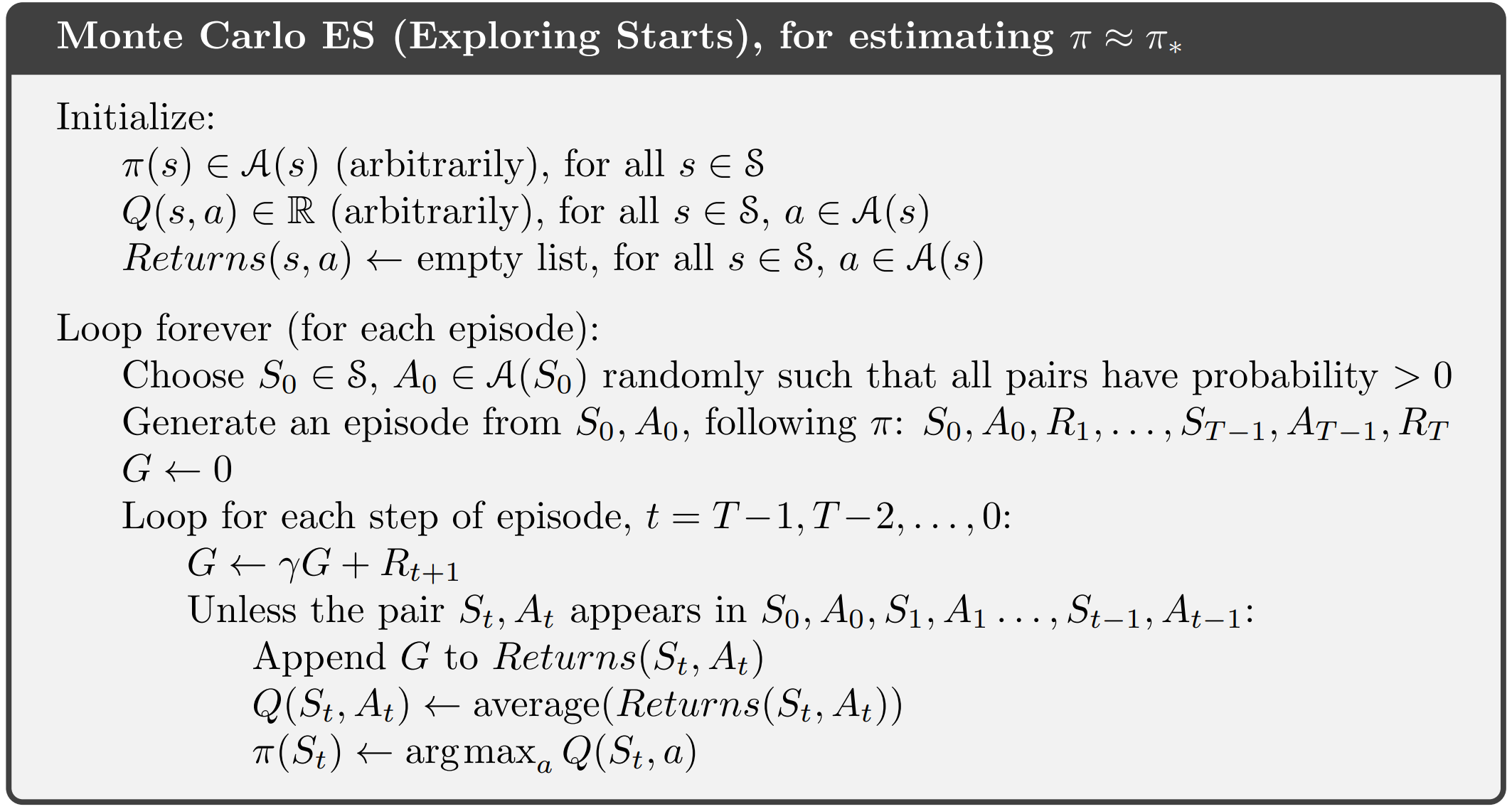
Exploring Starts
The pseudocode for exploring starts can be found below:
On-Policy First Visit MC Control
The pseudocode for On-Policy First Visit MC Control can be found below:
The python implementation for the following can be found below: This code is part of my collection of RL algorithms, that can be found in my GitHub repo drl-algorithms.
1
2
3
4
5
6
7
8
9
10
11
12
13
14
15
16
17
18
19
20
21
22
23
24
25
26
27
28
29
30
31
32
33
34
35
36
37
38
39
40
41
42
43
44
45
46
47
48
49
50
51
import gymnasium as gym
import numpy as np
env = gym.make('FrozenLake-v1', desc=None, map_name="8x8",
               is_slippery=False, render_mode="rgb_array")

action_values = np.zeros((env.observation_space.n,env.action_space.n))

def policy(state,epsilon=0.2):
    if np.random.random()<epsilon:
        return np.random.choice(env.action_space.n)
    else:
        action_value = action_values[state]
        return np.random.choice(np.flatnonzero(action_value == action_value.max()))

def on_policy_monte_carlo(policy,action_values,episodes,gamma=0.99,epsilon=0.2):
    sa_returns = {}

    for episode in range(1, episodes+1):
        state,info = env.reset()
        done = False
        transitions = []

        while not done:
            action = policy(state=state,epsilon=epsilon)
            next_state,reward,terminated,truncated,info = env.step(action=action)
            done = terminated or truncated
            transitions.append([state,action,reward])
            state = next_state

        G = 0

        for state_t,action_t,reward_t in reversed(transitions):
            G = reward_t + gamma*G

            if not (state_t,action_t) in sa_returns:
                sa_returns[(state_t,action_t)] = []
                sa_returns[(state_t,action_t)].append(G)
                action_values[state_t,action_t] = np.mean(sa_returns[(state_t,action_t)])
    env.close()


on_policy_monte_carlo(policy=policy,action_values=action_values,episodes=10000)

env = gym.make('FrozenLake-v1', desc=None, map_name="8x8",
               is_slippery=False, render_mode="human")
observation,info = env.reset()
terminated = False
while not terminated:
    action = policy(observation,epsilon=0)
    observation, reward, terminated, truncated, info = env.step(action=action)
env.close()
On-Policy Every Visit MC Control
On-Policy Every Visit MC Control can be implemented by making a small change to the inner loop of the above code for the first visit version as follows: This code is part of my collection of RL algorithms, that can be found in my GitHub repo drl-algorithms.
1
2
3
4
5
6
7
8
9
10
11
12
13
14
15
16
17
18
19
20
21
22
23
24
25
26
def on_policy_monte_carlo(policy,action_values,episodes,gamma=0.99,epsilon=0.2):
    sa_returns = {}

    for episode in range(1, episodes+1):
        state,info = env.reset()
        done = False
        transitions = []

        while not done:
            action = policy(state=state,epsilon=epsilon)
            next_state,reward,terminated,truncated,info = env.step(action=action)
            done = terminated or truncated
            transitions.append([state,action,reward])
            state = next_state

        G = 0

        for state_t,action_t,reward_t in reversed(transitions):
            G = reward_t + gamma*G

            if not (state_t,action_t) in sa_returns:
                sa_returns[(state_t,action_t)] = []
            sa_returns[(state_t,action_t)].append(G)
            action_values[state_t,action_t] = np.mean(sa_returns[(state_t,action_t)])
    env.close()
On-Policy Every Visit Constant Alpha MC Control
The constant alpha version is based on the idea of using a running mean instead of using a normal return to deal with non-stationary problems.
The major change being the following equation: \(Q(S_t|A_t) \leftarrow Q(S_t|A_t) + \alpha(G_t-Q(S_t|A_t))\)
The python implementation can be found below: This code is part of my collection of RL algorithms, that can be found in my GitHub repo drl-algorithms.
1
2
3
4
5
6
7
8
9
10
11
12
13
14
15
16
17
18
19
20
21
22
23
24
25
26
27
28
29
30
31
32
33
34
35
36
37
38
39
40
41
42
43
44
45
46
47
48
49
import gymnasium as gym
import numpy as np
env = gym.make('FrozenLake-v1', desc=None, map_name="8x8",
               is_slippery=False, render_mode="rgb_array")

action_values = np.zeros((env.observation_space.n,env.action_space.n))

def policy(state,epsilon=0.2):
    if np.random.random()<epsilon:
        return np.random.choice(env.action_space.n)
    else:
        action_value = action_values[state]
        return np.random.choice(np.flatnonzero(action_value == action_value.max()))

def constant_alpha_monte_carlo(policy,action_values,episodes,gamma=0.99,epsilon=0.2,alpha=0.2):

    for episode in range(1, episodes+1):
        state,info = env.reset()
        done = False
        transitions = []

        while not done:
            action = policy(state=state,epsilon=epsilon)
            next_state,reward,terminated,truncated,info = env.step(action=action)
            done = terminated or truncated
            transitions.append([state,action,reward])
            state = next_state

        G = 0

        for state_t,action_t,reward_t in reversed(transitions):
            G = reward_t + gamma*G

            old_value = action_values[state_t,action_t]
            action_values[state_t,action_t] += alpha*(G-old_value)

    env.close()


constant_alpha_monte_carlo(policy=policy,action_values=action_values,episodes=20000)

env = gym.make('FrozenLake-v1', desc=None, map_name="8x8",
               is_slippery=False, render_mode="human")
observation,info = env.reset()
terminated = False
while not terminated:
    action = policy(observation,epsilon=0)
    observation, reward, terminated, truncated, info = env.step(action=action)
env.close()
Off-Policy MC Control
In Off-Policy methods, the policy used to generate behavior, called the behavior policy, may in fact be unrelated to the policy that is evaluated and improved, called the target policy. An advantage of this separation is that the target policy may be deterministic (e.g., greedy), while the behavior policy can continue to sample all possible actions.
Off-policy Monte Carlo control methods use one of the techniques presented in the preceding two sections. They follow the behavior policy while learning about and improving the target policy. These techniques require that the behavior policy has a nonzero probability of selecting all actions that might be selected by the target policy (coverage). To explore all possibilities, we require that the behavior policy be soft (i.e., that it select all actions in all states with nonzero probability).
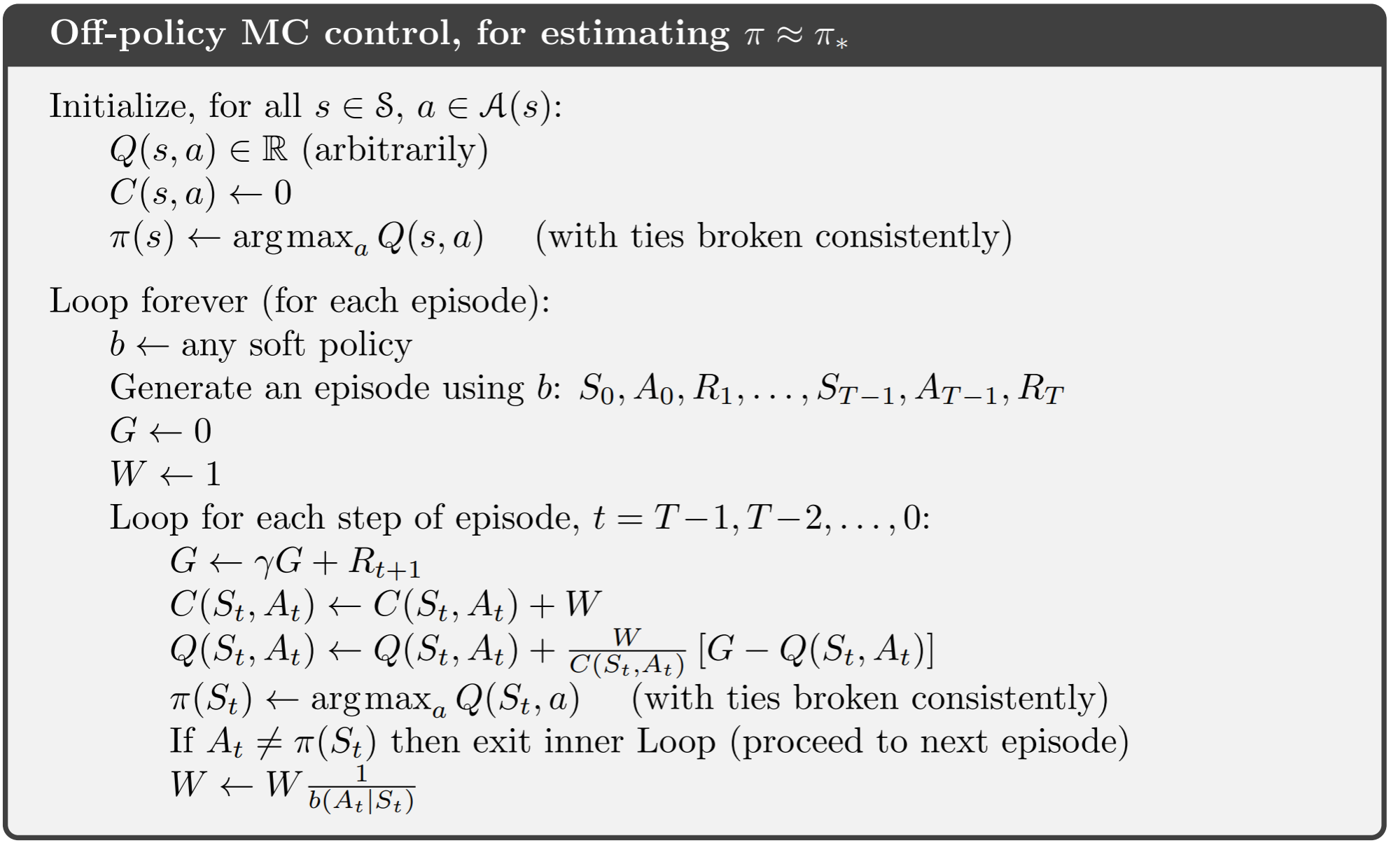
The python implementation of the above can be found here: This code is part of my collection of RL algorithms, that can be found in my GitHub repo drl-algorithms.
1
2
3
4
5
6
7
8
9
10
11
12
13
14
15
16
17
18
19
20
21
22
23
24
25
26
27
28
29
30
31
32
33
34
35
36
37
38
39
40
41
42
43
44
45
46
47
48
49
50
51
52
53
54
55
56
57
58
59
import gymnasium as gym
import numpy as np
env = gym.make('FrozenLake-v1', desc=None, map_name="8x8",
                is_slippery=False, render_mode="rgb_array")

action_values = np.zeros((env.observation_space.n,env.action_space.n))

def target_policy(state):
    action_value = action_values[state]
    return np.random.choice(np.flatnonzero(action_value == action_value.max()))

def exploratory_policy(state,epsilon=0.2):
    if np.random.random()<epsilon:
        return np.random.choice(env.action_space.n)
    else:
        action_value = action_values[state]
        return np.random.choice(np.flatnonzero(action_value == action_value.max()))


def off_policy_monte_carlo(action_values,target_policy,exploratory_ploicy,episodes,gamma=0.99,epsilon=0.2):
    counter_sa_values = np.zeros((env.observation_space.n,env.action_space.n))

    for episode in range(1,episodes+1):
        state,_ = env.reset()
        done = False
        transitions = []

        while not done:
            action = exploratory_ploicy(state=state,epsilon=epsilon)
            next_state,reward,terminated,truncated,_ = env.step(action=action)
            done = terminated or truncated
            transitions.append([state,action,reward])
            state = next_state

        G = 0
        W = 1

        for state_t,action_t,reward_t in reversed(transitions):
            G = reward_t + gamma*G
            counter_sa_values[state_t,action_t] += W
            old_value = action_values[state_t,action_t]
            action_values[state_t,action_t] += (W/counter_sa_values[state_t,action_t])* (G - old_value)

            if action_t != target_policy(state_t):
                break

            W = W*(1/(1-epsilon + (epsilon/4)))
    env.close()

off_policy_monte_carlo(action_values=action_values,target_policy=target_policy,exploratory_ploicy=exploratory_policy,episodes=5000)

env = gym.make('FrozenLake-v1', desc=None, map_name="8x8",
               is_slippery=False, render_mode="human")
observation,_ = env.reset()
terminated = False
while not terminated:
    action = target_policy(observation)
    observation, reward, terminated, truncated, info = env.step(action=action)
env.close()
Temporal Difference Methods
Temporal Difference methods improvise over MC methods by learning from incomplete episodes of experience using bootstrapping.
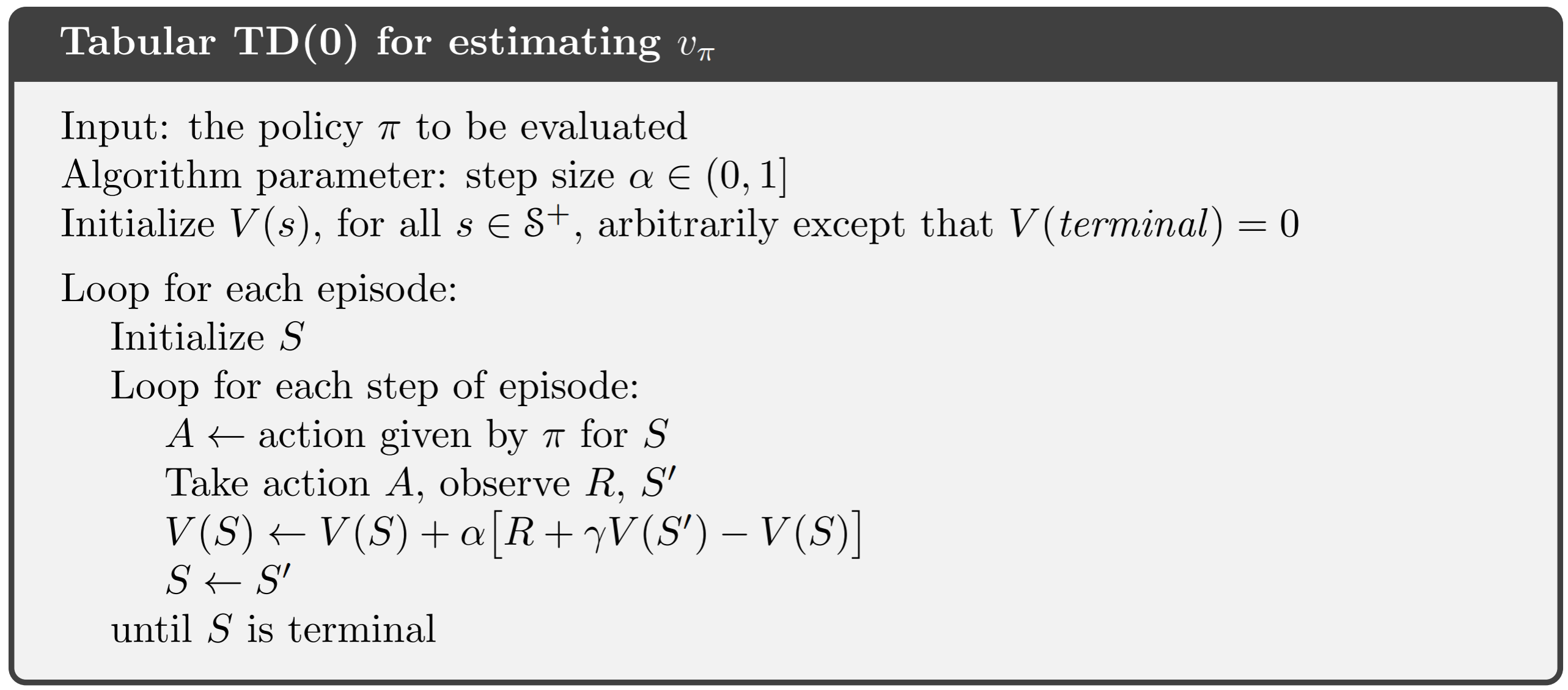
Temporal Difference Prediction
The simplest temporal-difference learning algorithm TD(0) works as follows:
The $V(S_t)$ can be updated using the actual return $G_t$
\[V(S_t) \leftarrow V(S_t) + \alpha(G_t - V(S_t))\]We can replace the actual return $G_t$ with the estimated return $R_{t+1} + \gamma V(S_{t+1})$ as follows
\[V(S_t) \leftarrow V(S_t) + \alpha(R_{t+1} + \gamma V(S_{t+1}) - V(S_t))\]Where,
$R_{t+1} + \gamma V(S_{t+1})$ is called the TD target
$\delta_t = R_{t+1} + \gamma V(S_{t+1}) - V(S_t) $ is called the TD error
On-Policy TD Prediction
On-Policy TD prediction can be implemented as explained below
Off-Policy TD Prediction
Using Importance Sampling for Off-Policy Learning, we can implement TD Prediction as follows:
Use TD targets generated from $\mu$ to evaluate $\pi$. We can weight the TD target $(R + \gamma V(S’))$ by the importance sampling ratio. Note that we only need to correct a single instane of the prediction unlike MC methods where the whole episde has to be corrected.
\[V(S_t) \leftarrow V(S_t) + \alpha \left( \dfrac{\pi(A_t|S_t)}{\mu(A_t|S_t)}(R_{t+1} + \gamma V(S_{t+1})) - V(S_t) \right)\]Note that the variance is much lower than MC importance sampling
Temporal Difference Control
The basic stratergy for using TD methods for control is to plug them into the GPI framework for policy evaluation by learning action values to remain model-free.
The general update rule for action value estimation can be written as:
\[Q(S_t,A_t) \leftarrow Q(S_t,A_t) + \alpha [R_{t+1} + \gamma Q(S_{t+1},A_{t+1}) - Q(S_t,A_t)]\]On-Policy TD Control (SARSA)
The On-Policy TD Control method is also referred to as SARSA as it uses the quintuple of events $(S_t,A_t,R_{t+1},S_{t+1},A_{t+1})$ for every update.
The pseudocode for SARSA can be found below
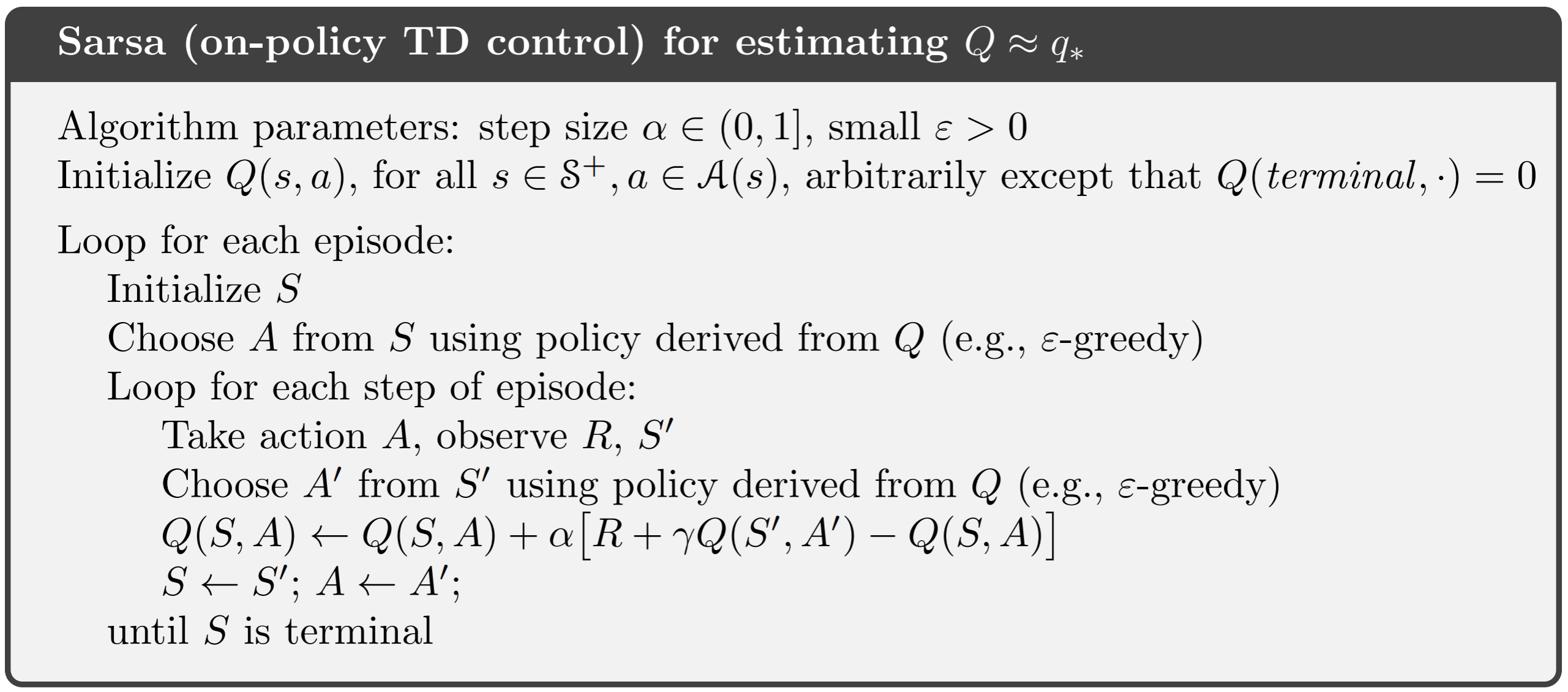
The python implementation of the above can be found here: This code is part of my collection of RL algorithms, that can be found in my GitHub repo drl-algorithms.
1
2
3
4
5
6
7
8
9
10
11
12
13
14
15
16
17
18
19
20
21
22
23
24
25
26
27
28
29
30
31
32
33
34
35
36
37
38
39
40
41
42
43
44
45
46
47
48
import gymnasium as gym
import numpy as np

env = gym.make('FrozenLake-v1', desc=None, map_name="8x8",
               is_slippery=False, render_mode="rgb_array")

action_values = np.zeros((env.observation_space.n, env.action_space.n))


def policy(state, epsilon=0.2):
    if np.random.random() < epsilon:
        return np.random.choice(env.action_space.n)
    else:
        action_value = action_values[state]
        return np.random.choice(np.flatnonzero(action_value == action_value.max()))


def sarsa(action_values, episodes, policy, alpha=0.1, gamma=0.99, epsilon=0.2):  # on-policy-td-learning
    for episode in range(episodes+1):
        state, _ = env.reset()
        action = policy(state=state, epsilon=epsilon)
        done = False

        while not done:
            next_state, reward, termination, truncation, _ = env.step(
                action=action)
            done = termination or truncation
            next_action = policy(state=next_state, epsilon=epsilon)

            action_value = action_values[state, action]
            next_action_value = action_values[next_state, next_action]
            action_values[state, action] = action_value + alpha * \
                (reward + gamma*next_action_value - action_value)
            state = next_state
            action = next_action
    env.close()


sarsa(action_values=action_values, episodes=1000, policy=policy)

env = gym.make('FrozenLake-v1', desc=None, map_name="8x8",
               is_slippery=False, render_mode="human")
observation, _ = env.reset()
terminated = False
while not terminated:
    action = policy(observation, epsilon=0)
    observation, reward, terminated, truncated, info = env.step(action=action)
env.close()
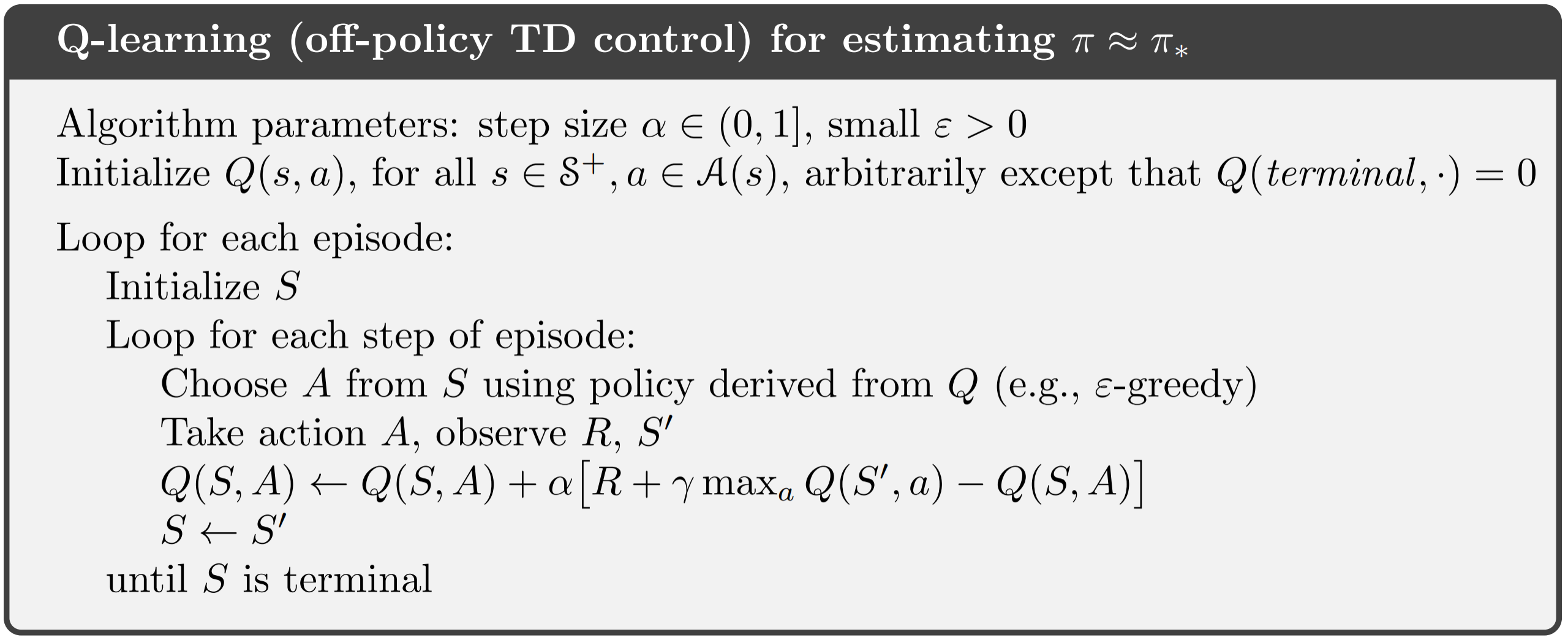
Off-Policy TD Control (Q-Learning)
Off-Policy TD Control is often referred to as Q-Learning and does not require importance sampling. For TD(0) based Q-Learning, since the action $A_t$ is already determined the importance sampling ratio essentially becomes 1 and therefore can be ignored.
The next action is chosen using a behaviour policy $A_{t+1} \sim \mu(.|S_t)$ which is $\epsilon$-greedy w.r.t $Q(S,A)$. But we consider alternative successor action $a \sim \pi(.|S_t)$ using the target policy $\pi$ which is greedy w.r.t $Q(S,A)$
The update rule can be written down as follows:
\[Q(S_t,A_t) \leftarrow Q(S_t,A_t) + \alpha[R_{t+1} + \gamma \mathtt{max}_{a} Q(S_{t+1},a) - Q(S_t,A_t)]\]The pseudocode for Q-Learning can be found below:
The python implementation of the above can be found here: This code is part of my collection of RL algorithms, that can be found in my GitHub repo drl-algorithms.
1
2
3
4
5
6
7
8
9
10
11
12
13
14
15
16
17
18
19
20
21
22
23
24
25
26
27
28
29
30
31
32
33
34
35
36
37
38
39
40
41
42
43
44
45
46
47
import gymnasium as gym
import numpy as np
env = gym.make('FrozenLake-v1', desc=None, map_name="8x8",
               is_slippery=False, render_mode="rgb_array")

action_values = np.zeros((env.observation_space.n, env.action_space.n))


def target_policy(state):
    action_value = action_values[state]
    return np.random.choice(np.flatnonzero(action_value == action_value.max()))


def exploratory_policy():
    return np.random.randint(env.action_space.n)


def q_learning(action_values, episodes, target_policy, exploratory_policy, alpha=0.1, gamma=0.99):  # on-policy-td-learning
    for episode in range(episodes+1):
        state, _ = env.reset()
        done = False

        while not done:
            action = exploratory_policy()
            next_state, reward, termination, truncation, _ = env.step(
                action=action)
            done = termination or truncation
            next_action = target_policy(state=next_state)

            action_value = action_values[state, action]
            next_action_value = action_values[next_state, next_action]
            action_values[state, action] = action_value + alpha * \
                (reward + gamma*next_action_value - action_value)
            state = next_state
    env.close()

q_learning(action_values=action_values, episodes=5000, target_policy=target_policy, exploratory_policy=exploratory_policy, alpha=0.1, gamma=0.99)

env = gym.make('FrozenLake-v1', desc=None, map_name="8x8",
               is_slippery=False, render_mode="human")
observation, _ = env.reset()
terminated = False

while not terminated:
    action = target_policy(observation)
    observation, reward, terminated, truncated, info = env.step(action=action)
env.close()
Expected SARSA
Consider the learning algorithm that is just like Q-learning except that instead of the maximum over next state–action pairs it uses the expected value, taking into account how likely each action is under the current policy. That is, consider the algorithm with the update rule as follows:
\[Q(S_t,A_t) \leftarrow Q(S_t,A_t) + \alpha[R_{t+1} + \gamma \mathbf{E}_\pi[Q(S_{t+1},A_{t+1} | S_{t+1})] - Q(S_t,A_t) ]\]which can be written as
\[Q(S_t,A_t) = Q(S_t,A_t) + \alpha[R_{t+1} + \gamma \Sigma_a\pi(a|S_{t+1})Q(S_{t+1},a) - Q(S_t,A_t) ]\]Expected Sarsa is more complex computationally than Sarsa but, in return, it eliminates the variance due to the random selection of At+1. Given the same amount of experience we might expect it to perform slightly better than Sarss.
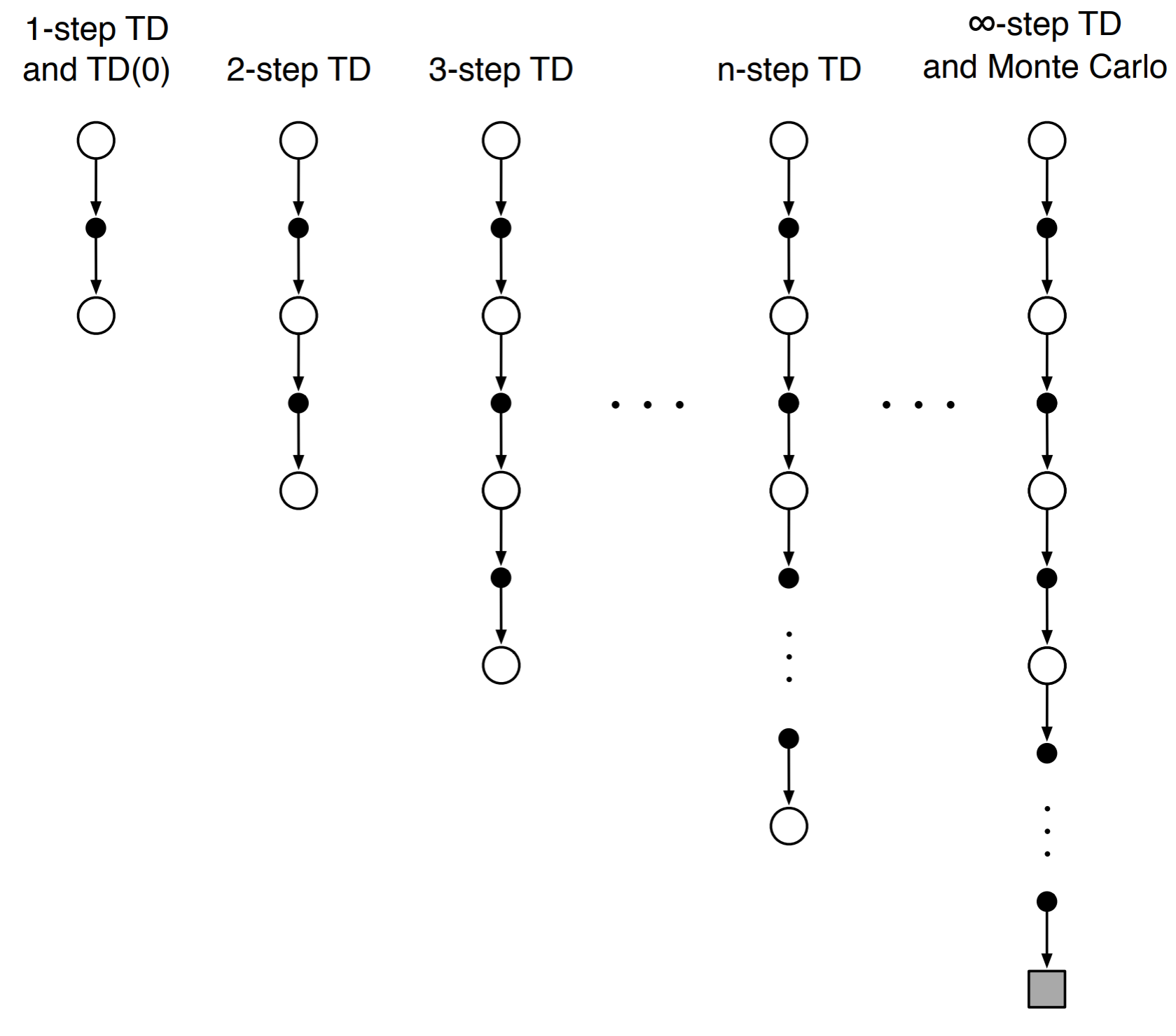
Bootstrapping
While TD(0) methods take one step and estimate the return, MC methods wait till the end of the episode to calculate the return. While both these methods might appear to be very different they can unified by using TD methods to look n-steps into the future, as shown by the image below.