
This post is part of the Deep Reinforcement Learning Blog Series. For a detailed introduction about the series, the curicullum, sources and references used, please check Part 0 - Getting Started.
Structure of the blog
- Part 0 - Getting Started
- Part 1 - Multi-Arm Bandits
- Part 2 - Finite MDP | Prerequisites: python, gymnasium, numpy
- Part 3 - Dynamic Programming | Prerequisites: python, gymnasium, numpy
- Part 4 - Monte Carlo, Temporal Difference & Bootstrapping Methods | Prerequisites: Python, gymnasium, numpy
- Part 5 - Deep SARSA and Q-Learning | Prerequisites: python, gymnasium, numpy, torch
- Part 6 - REINFORCE, AC, DDPG, TD3, SAC
- Part 7 - A2C, PPO, TRPO, GAE, A3C
- TBA (HER, PER, Distillation)
Dynamic Programming
The term dynamic programming (DP) refers to a collection of algorithms that can be used to compute optimal policies given a perfect model of the environment as a Markov decision process (MDP). Classical DP algorithms are of limited utility in reinforcement learning both because of their assumption of a perfect model and because of their great computational expense, but they are still important theoretically. DP provides an essential foundation for the understanding of the Approx. methods presented in later parts. In fact, all of these methods can be viewed as attempts to achieve much the same effect as DP, only with less computation and without assuming a perfect model of the environment.
Policy Evaluation
First we consider how to compute the state-value function $v_\pi$ for an arbitrary policy $\pi$. This is called policy evaluation in the DP literature. We also refer to it as the prediction problem.
Recall that,
\[v_\pi(s) = \sum_{a}\pi(a\mid s)\sum_{s',r} p(s',r\mid a,s)[r+\gamma v_\pi(s')]\]We can evaluate a given policy $\pi$ by iterativly applying the bellman expectation backup as an update rule until the value function $v(s)$ converges to the $v_\pi(s)$.
Policy Improvement
We can then improve a given policy by acting greedily with respect to the given value function for the policy $v_\pi(s)$.
The new policy $\pi’$ is better than or equal to the old policy $\pi$. Therefore, $\pi’ \ge \pi$.
If the improvement stops
\[q_\pi(s,\pi'(s)) = \mathtt{max}_{a \in A} \ q_\pi(s,a) \ = q_\pi(s,\pi(s)) = v_\pi(s)\]Therefore,
\[v_\pi(s) = \mathtt{max}_{a \in A} q_\pi(s,a)\]which is the bellman optimality equation and $v_\pi(s) = v_\star(s)$.
Policy Iteration
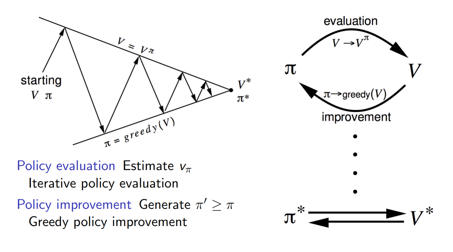
Policy Iteration combines the evaluation and improvement steps into a single algorithm where a random policy is taken, its evaluated and then improved upon and the resulting policy is again evaluated and then improved upon and so on until the policy finally converges and becomes the optimal policy.
Policy Iteration is also refered to as the control problem in DP litrature as opposed to the prediction problem that is policy evaluation.
The algorithm can be summaried as follows:
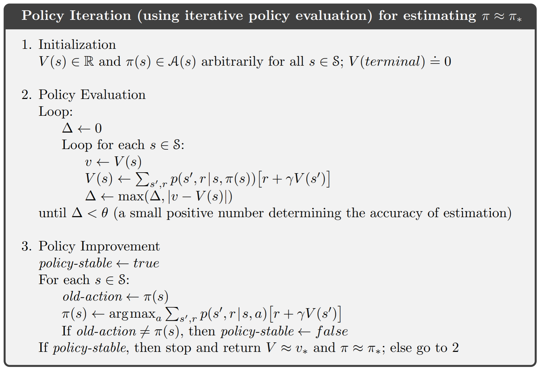
The $\Delta$ in the above code is used to determine the accuracy of the estimation and can be a value close to 0.
The python code for Policy Iteration is as follows:
This code is part of my collection of RL algorithms, that can be found in my GitHub repo drl-algorithms.
1
2
3
4
5
6
7
8
9
10
11
12
13
14
15
16
17
18
19
20
21
22
23
24
25
26
27
28
29
30
31
32
33
34
35
36
37
38
39
40
41
42
43
44
45
46
47
48
49
50
51
52
53
54
55
56
57
58
59
import gymnasium as gym
import numpy as np

env = gym.make('FrozenLake-v1', desc=None, map_name="8x8",
               is_slippery=False, render_mode="human")
observation, info = env.reset()
terminated = False

# state-action table
policy_probs = np.full((env.observation_space.n, env.action_space.n), 0.25)
state_values = np.zeros(shape=(env.observation_space.n))


def policy_iteration(policy_probs, state_values, theta=1e-6, gamma=0.99):
    policy_stable = False
    while policy_stable == False:
        # policy eval
        delta = 1
        while delta > theta:
            delta = 0
            for state in range(env.observation_space.n):
                old_value = state_values[state]
                new_state_value = 0
                for action in range(env.action_space.n):
                    probablity, next_state, reward, info = env.P[state][action][0]
                    new_state_value += policy_probs[state, action]*(
                        reward + (gamma*state_values[next_state]))
                state_values[state] = new_state_value
                delta = max(delta, abs(old_value-state_values[state]))
        # policy improvement
        policy_stable = True
        for state in range(env.observation_space.n):
            old_action = policy(state=state)
            action_values = np.zeros(env.action_space.n)
            max_q = float('-inf')
            for action in range(env.action_space.n):
                probablity, next_state, reward, info = env.P[state][action][0]
                action_values[action] = probablity * \
                    (reward + (gamma*state_values[next_state]))
                if action_values[action] > max_q:
                    max_q = action_values[action]
                    action_probs = np.zeros(env.action_space.n)
                    action_probs[action] = 1
            policy_probs[state] = action_probs
        # check termination condition and update policy_stable variable
            if old_action != policy(state=state):
                policy_stable = False


def policy(state):
    return np.argmax(policy_probs[state])


policy_iteration(policy_probs=policy_probs, state_values=state_values)
print("Done")
while not terminated:
    action = policy(observation)
    observation, reward, terminated, truncated, info = env.step(action=action)
env.close()
Another important point is the fact that we do not need to wait for the policy evaluation to converge to $v_\pi$ before performing policy improvement. Therefore, a stopping condition can be introduced without effecting the performance.
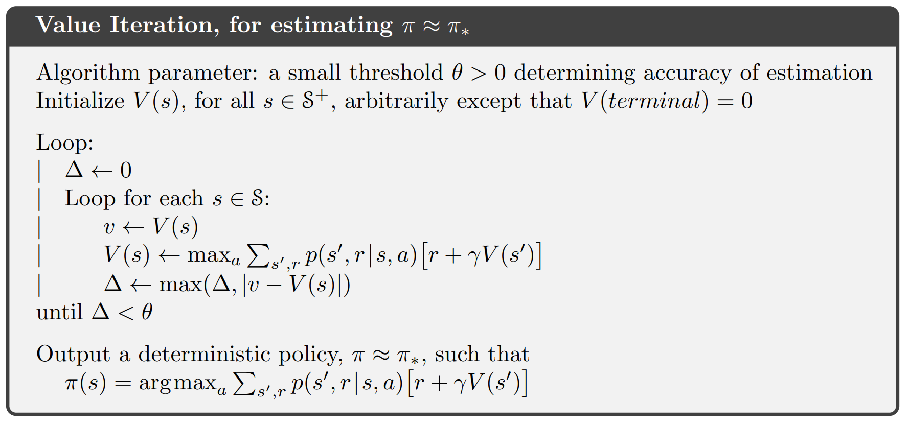
When the policy evaluation step is stopped after a single step, k = 1 we arrive at a special case of policy evaluation which is equivalent to another method called value iteration.
Value Iteration
The bellman optimality backup equation can be applied iteratively until convergence to arrive at the optimal value function $v_\star(s)$. Unlike policy iteration the itermediate value functions do not correspond to any policy. The algorithm can be summaried as follows:
 The python code for Value Iteration is as follows:
This code is part of my collection of RL algorithms, that can be found in my GitHub repo drl-algorithms.
1
2
3
4
5
6
7
8
9
10
11
12
13
14
15
16
17
18
19
20
21
22
23
24
25
26
27
28
29
30
31
32
33
34
35
36
37
38
39
40
41
42
43
44
45
46
import gymnasium as gym
import numpy as np

env = gym.make('FrozenLake-v1', desc=None, map_name="8x8",
               is_slippery=False, render_mode="human")

observation, info = env.reset()
terminated = False

# state-action table
policy_probs = np.full((env.observation_space.n, env.action_space.n), 0.25)
state_values = np.zeros(shape=(env.observation_space.n))


def value_iteration(policy_probs, state_values, theta=1e-6, gamma=0.99):
    delta = 1
    while delta > theta:
        delta = 0
        for state in range(env.observation_space.n):
            old_value = state_values[state]
            action_values = np.zeros(env.action_space.n)
            max_q = float('-inf')
            for action in range(env.action_space.n):
                probablity, next_state, reward, info = env.P[state][action][0]
                action_values[action] = probablity * \
                    (reward + (gamma*state_values[next_state]))
                if action_values[action] > max_q:
                    max_q = action_values[action]
                    action_probs = np.zeros(env.action_space.n)
                    action_probs[action] = 1
            state_values[state] = max_q
            policy_probs[state] = action_probs

            delta = max(delta, abs(old_value - state_values[state]))


def policy(state):
    return np.argmax(policy_probs[state])


value_iteration(policy_probs=policy_probs, state_values=state_values)

while not terminated:
    action = policy(observation)
    observation, reward, terminated, truncated, info = env.step(action=action)
env.close()
This code is part of my collection of RL algorithms, that can be found in my GitHub repo drl-algorithms.
| Problem | Bellman Equation | Algorithm |
|---|---|---|
| Prediction | Bellman Expectation Equation | Iterative Policy Evaluation |
| Control | Bellman Expectation Equation + Greedy Policy Improvement | Policy Iteration |
| Control | Bellman Optimality Equation | Value Iteration |
Async. Dynamic Programming
All the methods discussed till now were synchronous in nature and at each step of the iteration we used a loop to go over all the states. We can however also asynchronously backup states in any order and this will also lead to the same solution as long as all the states are selected atleast once. The added advantage is that this greatly reduces computational time and gives rise to methods like prioritised sweeping and others.
Generalized Policy Iteration
We use the term generalized policy iteration (GPI) to refer to the general idea of letting policy-evaluation and policy improvement processes interact, independent of the granularity and other details of the two processes. Almost all reinforcement learning methods are well described as GPI. That is, all have identifiable policies and value functions, with the policy always being improved with respect to the value function and the value function always being driven toward the value function for the policy. If both the evaluation process and the improvement process stabilize, that is, no longer produce changes, then the value function and policy must be optimal. The value function stabilizes only when it is consistent with the current policy, and the policy stabilizes only when it is greedy with respect to the current value function. Thus, both processes stabilize only when a policy has been found that is greedy with respect to its own evaluation function. This implies that the Bellman optimality equation holds, and thus that the policy and the value function are optimal.
Pros and Cons of Dynamic Programming
DP is sometimes thought to be of limited applicability because of the curse of dimensionality, the fact that the number of states often grows exponentially with the number of state variables. Large state sets do create diculties, but these are inherent difficulties of the problem, not of DP as a solution method. In fact, DP is comparatively better suited to handling large state spaces than competing methods such as direct search and linear programming.
But DP methods assume we know the dynamics of the environment which is one of the biggest limiting factors for their direct use in many cases. In the upcoming parts we will loot at methods that tackle this issue.