This post is part of the Deep Reinforcement Learning Blog Series. For a detailed introduction about the series, the curicullum, sources and references used, please check Part 0 - Getting Started.

Structure of the blog

• Part 0 - Getting Started
• Part 1 - Multi-Arm Bandits
• Part 2 - Finite MDP | Prerequisites: python, gymnasium, numpy
• Part 3 - Dynamic Programming | Prerequisites: python, gymnasium, numpy
• Part 4 - Monte Carlo, Temporal Difference & Bootstrapping Methods | Prerequisites: Python, gymnasium, numpy
• Part 5 - Deep SARSA and Q-Learning | Prerequisites: python, gymnasium, numpy, torch
• Part 6 - REINFORCE, AC, DDPG, TD3, SAC
• Part 7 - A2C, PPO, TRPO, GAE, A3C
• TBA (HER, PER, Distillation)

Finite MDP

We will now consider problems that involve evaluative feedback, as in bandits, but also an associative aspect—choosing different actions in different situations.

MDPs are a classical formalization of sequential decision making, where actions influence not just immediate rewards, but also subsequent situations, or states, and through those future rewards. Thus MDPs involve delayed reward and the need to trade off immediate and delayed reward.

In bandit problems we estimated the value $q_{\star}(a)$ of each action $a$, in MDPs we estimate the value $q_\star(s, a)$ of each action $a$ in each state $s$, or we estimate the value $v_\star(s)$ of each state given optimal action selections. These state-dependent quantities are essential to accurately assigning credit for long-term consequences to individual action selections.

MDP Framework

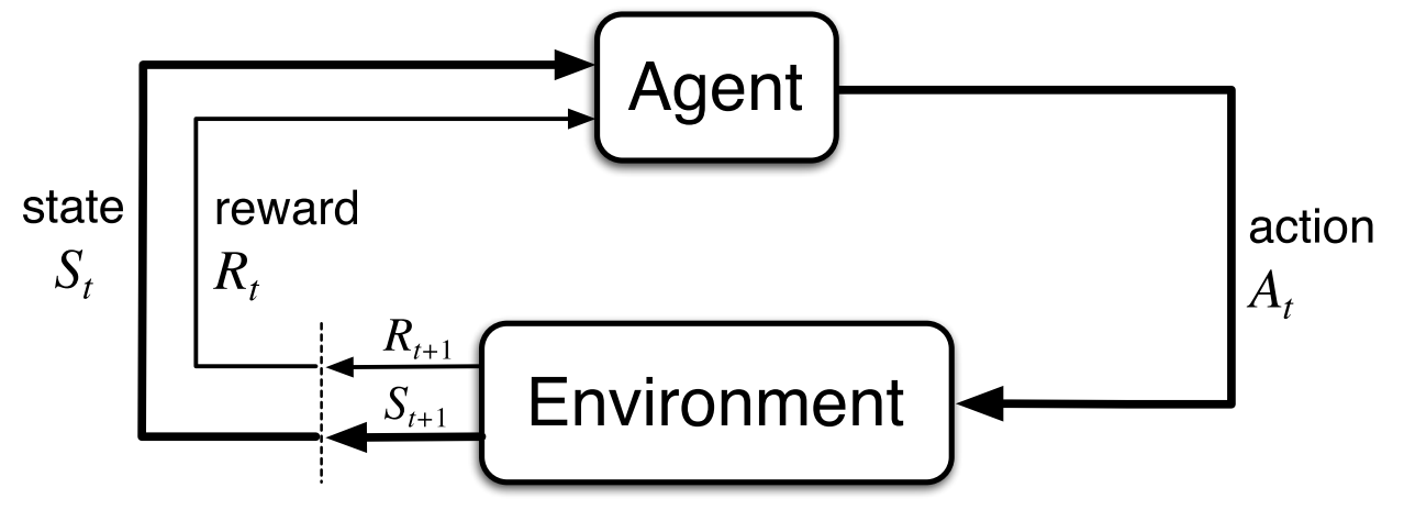In the above figure, the Agent is the learner and decision maker. Everything other than the agent is called the environmnet.

The agent and the environmnet interact with each other at every discrete timestep $t=0,1,2,..$ at each timestep the agent receives some representation of the environment’s state $S_t \in \mathit{S}$, and on that basis selects an action $A_t \in \mathit{A}(s)$ and one timestep later the environment responds to this action and presents a new state $S_{t+1}$ to the agent along with a numerical value called reward $R_{t+1} \in \mathit{R} \subset \mathbb{R}$ which the agent seeks to maximize over time through its choice of actions.

Taking the Cliff-Walking environment as an example, here is how we can access information about the state and observation space in gymnasium.

1
2
3
4
5
6
7
8
9

import gymnasium as gym

env = gym.make("CliffWalking-v0", render_mode="human")

observation, info = env.reset(seed=42)
print(f"The initial state after reset is : {observation}")
print(f"The State space is of the type: {env.observation_space}")
print(f"The Action space is of the type: {env.action_space}")
env.close()

The output for the above program is as follows:

1
2
3

The initial state after reset is : 36
The State space is of the type: Discrete(48)
The Action space is of the type: Discrete(4)

The MDP and agent together thereby give rise to a sequence or trajectory that begins like this:

The following is the python implementation for generating a trajectory for N=5 steps in the Cliff Walking Env

1
2
3
4
5
6
7
8
9
10
11
12
13
14
15
16
17

import gymnasium as gym

env = gym.make("CliffWalking-v0", render_mode="human")

observation, info = env.reset(seed=42)
trajectory = []

for _ in range(5):
    action = env.action_space.sample()
    new_observation,reward,terminated,truncated,info = env.step(action=action)
    trajectory.append([observation,action,reward])
    observation=new_observation
    
    if terminated or truncated:
        observation, info = env.reset()
env.close()
print(f"The Trajectory for 5 steps is: {trajectory}")

The output of the above program is as follows:

1

The Trajectory for 5 steps is: [[36, 3, -1], [36, 3, -1], [36, 3, -1], [36, 2, -1], [36, 0, -1]]

The above code can be slightly modified to generate the trajectory for an entire episode as follows:

1
2
3
4
5
6
7
8
9
10
11
12
13
14

import gymnasium as gym

env = gym.make("CliffWalking-v0",render_mode="rgb_array")

observation,info = env.reset(seed=42)
terminated = False
trajectory = []
while not terminated:
    action = env.action_space.sample()
    new_observation,reward,terminated,truncated,info = env.step(action=action)
    trajectory.append([observation,action,reward])
    observation = new_observation
env.close()
print(f"Trajectory for entire episode: {trajectory}")

In a finite MDP, the sets of states, actions, and rewards ($\mathit{S}$, $\mathit{A}$, and $\mathit{R}$) all have a finite number of elements. In this case, the random variables $R_t$ and $S_t$ have well defined discrete probability distributions dependent only on the preceding state and action. That is, for particular values of these random variables, $s’ \in \mathit{S}$ and $r \in \mathit{R}$, there is a probability of those values occurring at time t, given particular values of the preceding state and action:

Further since p specifies a probability distribution for each choice of s and a,

In a Markov decision process, the probabilities given by $p$ completely characterize the environment’s dynamics. That is, the probability of each possible value for $S_t$ and $R_t$ depends on the immediately preceding state and action, $S_{t-1}$ and $A_{t-1}$, and, given them, not at all on earlier states and actions. Therefore the state must include information about all aspects of the past agent–environment interaction that make a difference for the future. If it does, then the state is said to have the Markov property.

From the four-argument dynamics function, $p$, one can compute anything else one might want to know about the environment, such as

State-Transition Probabilities

A three-argument function denoting the probability of reaching state $s’$ when action $a$ is taken from state $s$.

Expected Reward for State-Action

A two-argument function defining the expected rewards for a state-action pair.

Expected Reward for State-Action-State

A Three argument function defining the expected rewards for a state-action-state pair.

Goals & Rewards

In reinforcement learning, the purpose or goal of the agent is formalized in terms of a special signal, called the reward, passing from the environment to the agent. At each time step, the reward is a simple number, $R_t \in \mathit{R}$. Informally, the agent’s goal is to maximize the total amount of reward it receives. This means maximizing not immediate reward, but cumulative reward in the long run.

The reward signal is your way of communicating to the agent what you want achieved, not how you want it achieved..

The Reward Hypothesis That all of what we mean by goals and purposes can be well thought of as the maximization of the expected value of the cumulative sum of a received scalar signal (called reward).

Returns & Episodes

To formally define how we wish to maximize the cumulative reward, we seek to maximize the expected return, where the return, denoted $G_t$,is defined as some specific function of the reward sequence. In the simplest case the return is the sum of the rewards:

Where T is the final timestep, this approach is applicable when there is a natural notion of final time step, that is, when the agent–environment interaction breaks naturally into subsequences, which we call episodes. Each episode ends in a special state called the terminal state, followed by a reset to a standard starting state or to a sample from a standard distribution of starting states. Even if you think of episodes as ending in different ways, such as winning and losing a game, the next episode begins independently of how the previous one ended. Thus the episodes can all be considered to end in the same terminal state, with different rewards for the different outcomes.

Tasks with episodes of this kind are called episodic tasks. In episodic tasks we sometimes need to distinguish the set of all nonterminal states, denoted $S$, from the set of all states plus the terminal state, denoted $S^+$. The time of termination, $T$, is a random variable that normally varies from episode to episode.

On the other hand, in many cases the agent–environment interaction does not break naturally into identifiable episodes, but goes on continually without limit. For example,this would be the natural way to formulate an on-going process-control task, or an application to a robot with a long life span. We call these continuing tasks. The return formulation discussed above is problematic for continuing tasks because the final time step would be $T = \infty$, and the return, which is what we are trying to maximize, could easily be infinite.

The additional concept that we need is that of discounting. According to this approach, the agent tries to select actions so that the sum of the discounted rewards it receives over the future is maximized. In particular, it chooses $A_t$ to maximize the expected discounted return:

Where $\gamma$ is called the discount factor and lies between $[0,1]$. The above formula can also be written recursivly as,

Unified Notation for Tasks

We need one other convention to obtain a single notation that covers both episodic and continuing tasks. We have defined the return as a sum over a finite number of terms in one case and as a sum over an infinite number of terms in the other. These two can be unified by considering episode termination to be the entering of a special absorbing state that transitions only to itself and that generates only rewards of zero. For example, consider the state transition diagram: 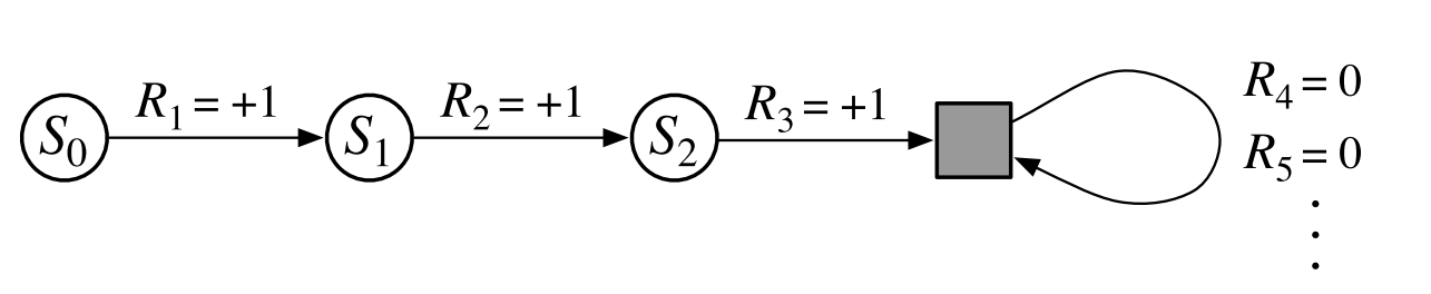Here the solid square represents the special absorbing state corresponding to the end of an episode. Starting from $S_0$, we get the reward sequence +1, +1, +1, 0, 0, 0,. …Summing these, we get the same return whether we sum over the first $T$ rewards (here $T$ = 3) or over the full infinite sequence. This remains true even if we introduce discounting.

We can therefore write the expected return as,

Where there is a possibilty that $T = \infty$ or $\gamma = 1$ (but not both).

The above formula can be used in code as follows:

1
2
3
4
5
6
7
8
9
10
11
12
13
14
15

import gymnasium as gym 

env = gym.make("CliffWalking-v0",render_mode="rgb_array")
terminated = False
G = 0 # Return 
observation, info = env.reset(seed=42)
counter = 0
gamma = 1
while not terminated:
    action = env.action_space.sample()
    observation,reward,terminated,truncated,info = env.step(action=action)
    G += reward*(gamma**counter)
    counter +=1
env.close()
print(f"The episode terminated after {counter} steps with Return(G) {G} for gamma {gamma}")

The output for the above code with various values of gamma is as follows:

1
2
3
4
5

The episode terminated after 853 steps with Return(G) -8575 for gamma 1

The episode terminated after 1391 steps with Return(G) -1445.9837656301004 for gamma 0.99

The episode terminated after 4516 steps with Return(G) -1 for gamma 0

Policies & Value Functions

Almost all reinforcement learning algorithms involve estimating value functions— which are functions of states (or of state–action pairs) that estimate how good it is for the agent to be in a given state (or how good it is to perform a given action in a given state).

The notion of “how good” here is defined in terms of future rewards that can be expected, or, to be precise, in terms of expected return. Of course the rewards the agent can expect to receive in the future depend on what actions it will take. Accordingly, value functions are defined with respect to particular ways of acting, called policies.

Formally, a policy is a mapping from states to probabilities of selecting each possible action. If the agent is following policy $\pi$ at time $t$,then $\pi(a\mid s)$ is the probability that $A_t = a$ if $S_t = s$. Like $p,\pi$ is an ordinary function.

The $\mid$ in the middle of $\pi(a\mid s)$ merely reminds us that it defines a probability distribution over $a \in \mathit{A}(s)$ for each $s \in \mathit{S}$. Reinforcement learning methods specify how the agent’s policy is changed as a result of its experience.

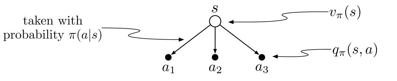
State Value Function

The value function of a state $s$ under a policy $\pi$, denoted by $v_\pi(s)$, is the expected return when starting in $s$ and following $\pi$ thereafter. For MDPs, we can define $v_\pi$ formally as

where $\mathbb{E}[.]$ denotes the expected value of the variable given that the agent follows the policy $\pi$. Also, the value of the terminal state is considered to be zero.

Action Value Function

The value of taking action $a$ in state $s$ under a policy $\pi$, denoted by $q_\pi(s, a)$, as the expected return starting from $s$, taking the action $a$, and thereafter following policy $\pi$:

Bellman Value Equations

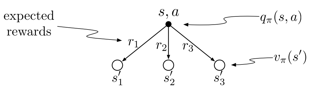
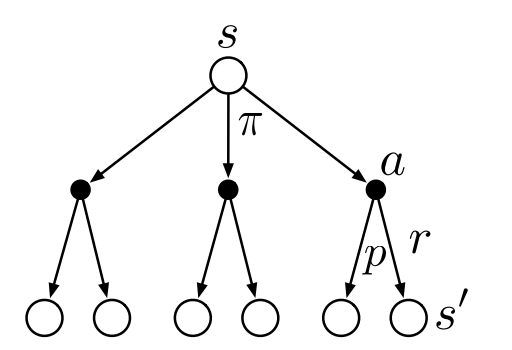
Substuting equation (2.2) in (2.1) we get the following recursive relation in terms of $v_\pi.$

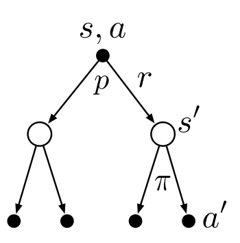
Substuting equation (2.1) in (2.2) we get the following recursive relation in terms of $q_\pi.$

Optimal Policies & Value Functions

There is always at least one policy that is better than or equal to all other policies. This is an optimal policy. Although there may be more than one, we denote all the optimal policies by $\pi_{\star}$. They share the same state-value function, called the optimal state-value function, denoted $v_\star$.

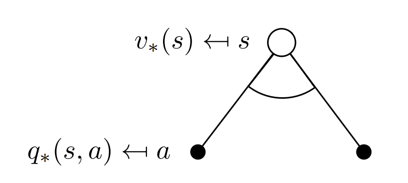
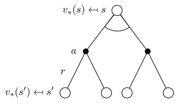
Substuting equation (2.5) in (2.4) we get the following recursive relation in terms of $v_\pi.$

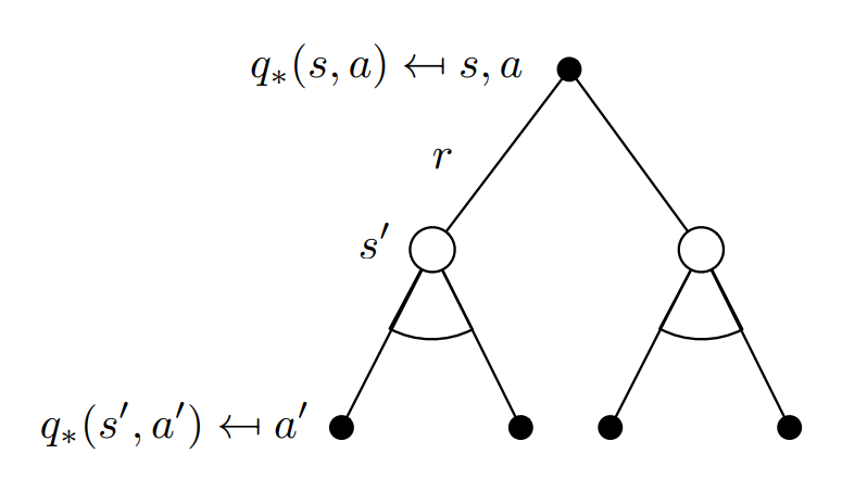
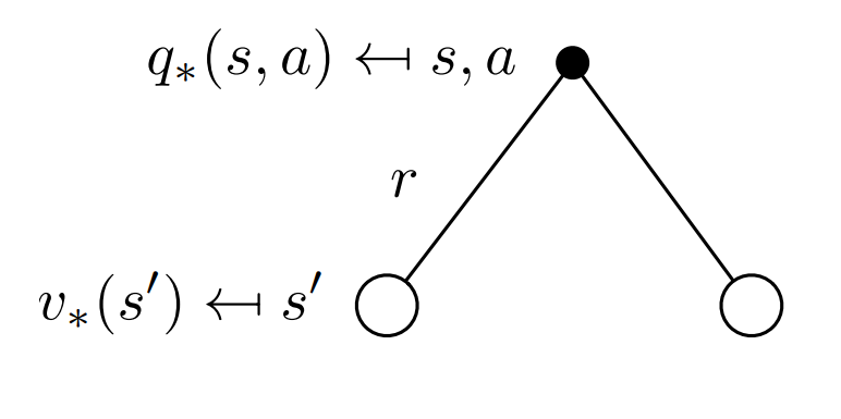
Substuting equation (2.4) in (2.5) we get the following recursive relation in terms of $q_\pi.$