Introduction
I wrote this small script to tinker with DH Parameters and wanted to visualize and understand how joint limits affect the manipulator workspace. While there are many ways of generating the workspace of a manipulator, this particular sketch uses forward kinematics to do so. The full code for the project can be found in the following repo

Method
The idea of plotting workspace from forward kinematics can be broken down into the following smaller tasks
- Capture the DH Table from the user
- Create a Homogenous Transformation Matrix ideally(Base to Tool).
- Take in user inputs for joint limits.
- Create a dataset of sorts that contains random possible combinations from the possible joint limits.
- Plug these random points into the Transformation Matrix and plot the outputs.
A few other points:
- There is no need to create a dataset with “all” possible combinations for the joint angles, this method will be computationally expensive. We will instead be using monte carlo distribution to generate random points.
- Angle limits for roll joint at the end of the tool tip need not be considered as change in roll values doesn’t change the tool tip position.
The Code Explanined
Capture the DH Table from the user
The first step would be to capture the DH-Parameters for a given manipulators, this can be represented using a “M x 4 matrix” where M is the number of axis for the manipulator.
We will be creating a matrix using symbolic variables as it would make it easier later for us to solve the matrix multiplications using variables that can later be substituted for.
1
2
3
4
5
%% Homogeneous Matrix Builder
noParams = input('Enter the number of axis: ');
T = [1,0,0,0;0,1,0,0;0,0,1,0;0,0,0,1];
flg = [0,0,0,0];
A = sym('A%d%d',[noParams,4]);
noParams here is used to decide the number of rows for the DH parameter table. A is the DH-Table Matrix
On its own for an input of “5” to noParams, the A matrix would look like this:
1
2
3
4
5
6
7
8
9
>> A

A =

[A11, A12, A13, A14]
[A21, A22, A23, A24]
[A31, A32, A33, A34]
[A41, A42, A43, A44]
[A51, A52, A53, A54]
The names of the column and row elements are due to the “A%d%d” in the A = sym('A%d%d',[noParams,4]);
Create a Homogenous Transformation Matrix ideally(Base to Tool).
We will now be creating a Homogenous symbolic transformation matrix with the above generated blank DH paramter matrix.
- Rotation of $L_{k-1}$ about $Z_{k-1}$ is denoted by $\theta_k$.
- Translation of $L_{k-1}$ about $Z_{k-1}$ is denoted by $d_k$.
- Translation of $L_{k-1}$ about $X_{k-1}$ is denoted by $a_k$.
- Rotation of $L_{k-1}$ about $X_{k-1}$ is denoted by $\alpha_k$.
Therefore, any homogenous Transformation matrix T can be expressed as the following:
\(T_{k-1}^k(\theta_k,d_k,a_k,\alpha_k) = R(\theta_k,z)T(d_k,z)T(a_k,x)R(\alpha_k,x)\)
\(T_{base}^{tool} = T_{base}^1T_1^2T_2^3...T_{n-1}^{tool}\)
1
2
3
4
5
6
7
for i=1:1:noParams
  Rz = [cos(A(i,1)),-sin(A(i,1)),0,0;sin(A(i,1)),cos(A(i,1)),0,0;0,0,1,0;0,0,0,1];
  Tz = [1,0,0,0;0,1,0,0;0,0,1,A(i,2);0,0,0,1];
  Tx = [1,0,0,A(i,3);0,1,0,0;0,0,1,0;0,0,0,1];
  Rx = [1,0,0,0;0,cos(A(i,4)),-sin(A(i,4)),0;0,sin(A(i,4)),cos(A(i,4)),0;0,0,0,1];
  T = T*(Rz*Tz*Tx*Rx);
end
The next step after generating the DH table would be to fill the empty Transformation Matrix with the acutal values for the manipulator, this is done via user input.
This part of the code isn’t that straightforward, we will be taking one DH parameter at a time and the user needs to enter the row and column number of the DH paramter they are about to enter. The syntax for user input is [position,value,1/0]. Where a 1 would mean its the end of the inputs series and there are no more DH paramters to input, on the other hand 0 can be used to let the program know that there are more DH paramters that need to be entered.
NOTE:
- Users only need to enter DH-Paramters that are constant like “link length” and other values that cannot change.
1
2
3
4
5
6
while flg(4) == 0
        flg=input('Enter data as [position,value,1/0]: '); %constants filler
        T = vpa(subs(T,A(flg(1),flg(2)),flg(3)),4);
    end
	disp('Tool to Base Transformation Matrix created');
    disp(T);
After the Homogenous Transformation matrix is created, we can extract the tool-tip cordinate equations and convert them into a function so that we can substitue numerical values into the variables to get the tool tip postion.
1
2
Tpos=[T(1,4),T(2,4),T(3,4)];
Tpost = matlabFunction(Tpos);
matlabFunction is used to convert symbolic expressions into matlab function handles.
Take in user inputs for joint limits
We will now be taking in user inputs for joint limits and create a dataset with random combinations of joint angles using monte carlo.
- lim contains all the random datasets generated.
- N=67312 is the number of random combinations that will be generated, this number can be increased or decresed based on the needs, remember that the higher the number the more dense the workspace plot will turn out, but it will also increase the computation time.
Dataset = lower limit + (upper limit - lower limit)*random number between 0 and 1
1
2
3
4
5
6
7
8
9
ch2=input('Press 1 if you want to plot the 3D workspace');
    if ch2 == 1
        N = 67312;
        range=input('Enter upper and lower limits of each joint. EXCLUDE ROLL JOINTS');
        lim(N,size(range,1))=0;
        for i=1:size(range,1)
            lim(:,i) = range(i,1) + (range(i,2)-range(i,1))*rand(N,1);
        end
    end
Creating a dataset of points
There is nothing much to explain here, we are just iterating through all the possible combinations of numbers that we generated and are storing them in f
1
2
3
4
5
6
7
8
9
10
11
12
13
14
15
16
17
18
19
20
21
22
23
24
25
26
27
28
29
30
31
32
33
34
35
%% Plot Points Collector
    f(size(lim,1),3) = 0;
    if size(range,1) == 2
        for j=1:size(lim,1)
            f(j,:)=Tpost(lim(j,1),lim(j,2));
        end
    elseif size(range,1) == 3
        for j=1:size(lim,1)
            f(j,:)=Tpost(lim(j,1),lim(j,2),lim(j,3));
        end
    elseif size(range,1) == 4
        for j=1:size(lim,1)
            f(j,:)=Tpost(lim(j,1),lim(j,2),lim(j,3),lim(j,4));
        end
    elseif size(range,1) == 5
        for j=1:size(lim,1)
            f(j,:)=Tpost(lim(j,1),lim(j,2),lim(j,3),lim(j,4),lim(j,5));
        end
    elseif size(range,1) == 6
        for j=1:size(lim,1)
            f(j,:)=Tpost(lim(j,1),lim(j,2),lim(j,3),lim(j,4),lim(j,5),lim(j,6));
        end
    elseif size(range,1) == 7
        for j=1:size(lim,1)
            f(j,:)=Tpost(lim(j,1),lim(j,2),lim(j,3),lim(j,4),lim(j,5),lim(j,6),lim(j,7));
        end
    elseif size(range,1) == 8
        for j=1:size(lim,1)
            f(j,:)=Tpost(lim(j,1),lim(j,2),lim(j,3),lim(j,4),lim(j,5),lim(j,6),lim(j,7),lim(j,8));
        end
    elseif size(range,1) == 9
        for j=1:size(lim,1)
            f(j,:)=Tpost(lim(j,1),lim(j,2),lim(j,3),lim(j,4),lim(j,5),lim(j,6),lim(j,7),lim(j,8),lim(j,9));
        end
    end
Plotting Points
While the plot is 3D we will plot a few standard views as moving the plot around when it is extremly dense is a computationally heavy task.
1
2
3
4
5
6
7
8
9
10
11
12
13
14
15
16
17
18
19
20
21
22
%% Workspace Plotter
disp('Starting Workspace Plotter');
for i=1:N
plot3(f(i,1),f(i,2),f(i,3),'.')
hold on;
end
view(3);
title('Isometric view');
xlabel('x (m)');
ylabel('y (m)');
zlabel('z (m) ');
view(2); % top view
title(' Top view');
xlabel('x (m)');
ylabel('y (m)');
view([0 1 0]); % y-z plane
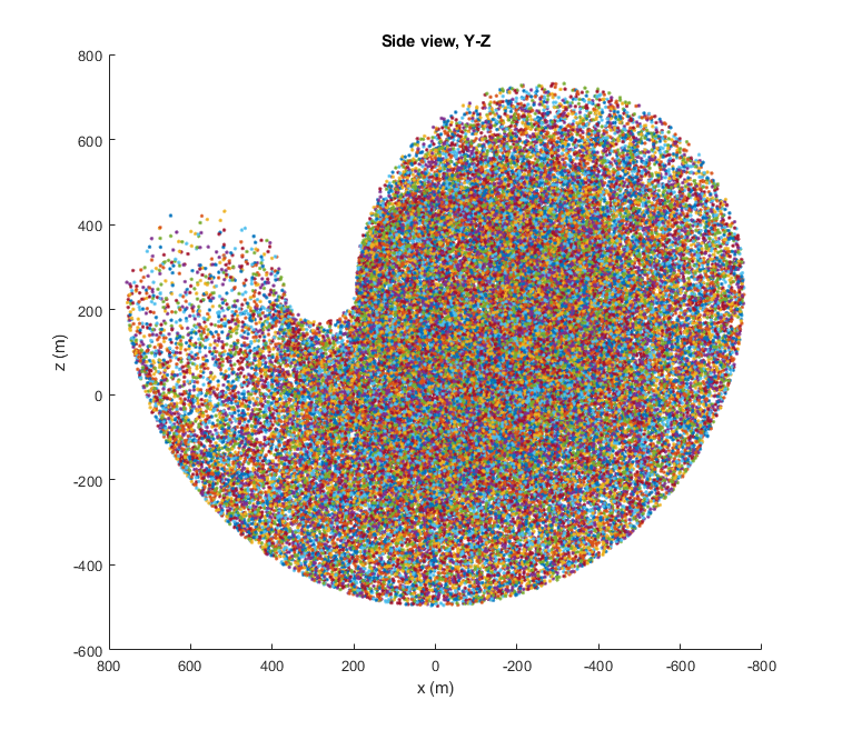
title('Side view, Y-Z');
ylabel('y (m)');
zlabel('z (m)');
disp('Plotting Complete');
NOTE
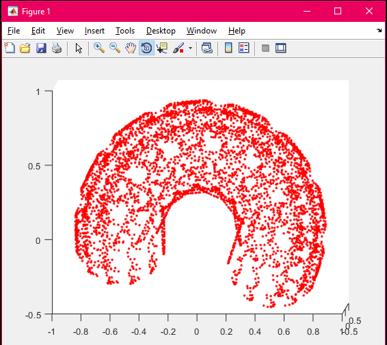
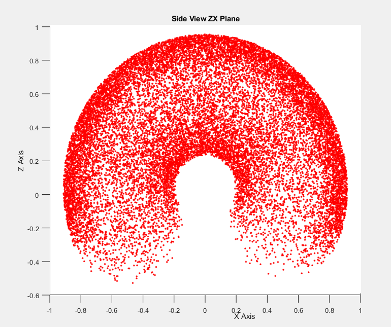
This version of the documentation is based on the DHPnP_v1.m which is based on the monte carlo method for random point sampling. The older version of the same project is based on a different approach and is significantly slower and more computational expenseive and memory intensive.
Results
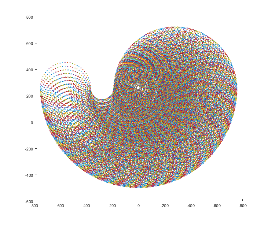
A few images from both the versions which clearly shows the difference in the resulting workspace plots.