Introduction
Coordinate Transformation in 2D
The motion of manipulators and robots is often very complex and mathematically demanding. A single coordinate frame usually isn’t sufficient, and its often convenient to use multiple coordinate frames (fixed or moving) to make things easier.
Terminology
Fixed and World coordinate frames are used interchangeably and mean the same thing.
Mobile and Moving coordinate frames are used interchangeably and mean the same thing.
What is a Coordinate Frame ?
If $p$ is a vector in $R^n$ and $X = {x^1 , x^2 , …x^n}$ be a complete orthonormal set of $R^n$, then coordinates of $p$ with respect to $X$ are denoted as $[p]^x$.
\[\begin{aligned} p &= \Sigma{[p]_k^x}\hat{x^k} \\ [p]_k^x &= p.x^k \end{aligned}\]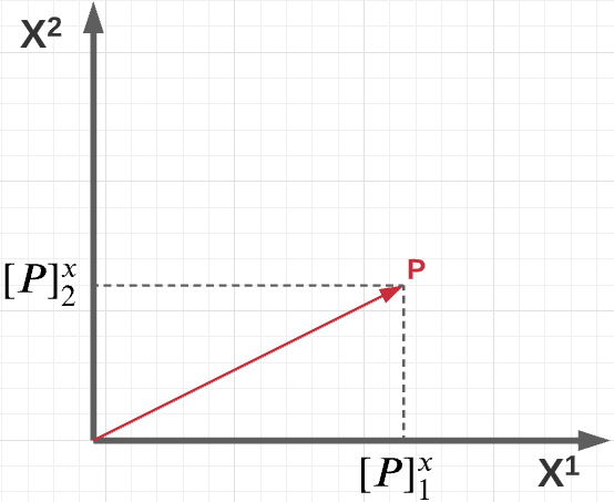
Translation
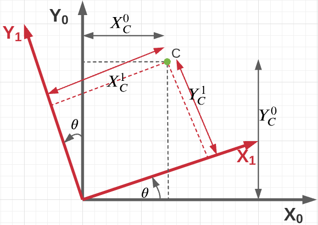
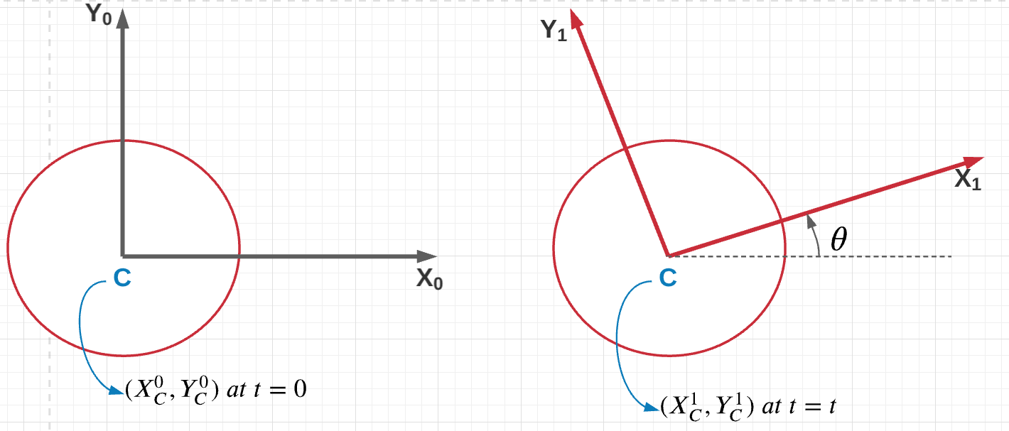
Assume a fixed frame $(O_0 − X_0 − Y_0 )$ and a mobile frame $(O_1 − X_1 − Y_1 )$. Let $C$ be a point in space. The relation between both the frames and $C$ can be derived using simple math.
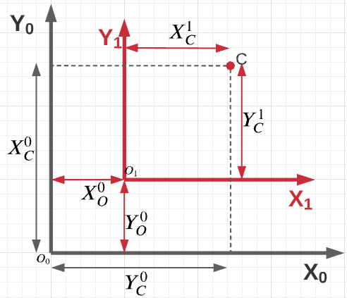
The following inferences can be made from the above figure:
Position of C $\mathit{wrt}$ frame $(O_0-X_0-Y_0)$ can be represented as
Position of C $\textit{wrt}$ frame $(O_1-X_1-Y_1)$ can be represented as
\[\begin{equation*} C^1 = \begin{bmatrix} X_C^1\\ Y_C^1 \end{bmatrix} \end{equation*}\]Position of $O_1$ $\textit{wrt}$ frame $(O_0-X_0-Y_0)$ can be represented as
\[\begin{equation*} O_1^0 = \begin{bmatrix} X_0\\ Y_0 \end{bmatrix} \end{equation*}\]Position of $O_0$ $\textit{wrt}$ frame $(O_1-X_1-Y_1)$ can be represented as
\[\begin{equation*} O_0^1 = \begin{bmatrix} -X_0\\ -Y_0 \end{bmatrix} \end{equation*}\]Rotation
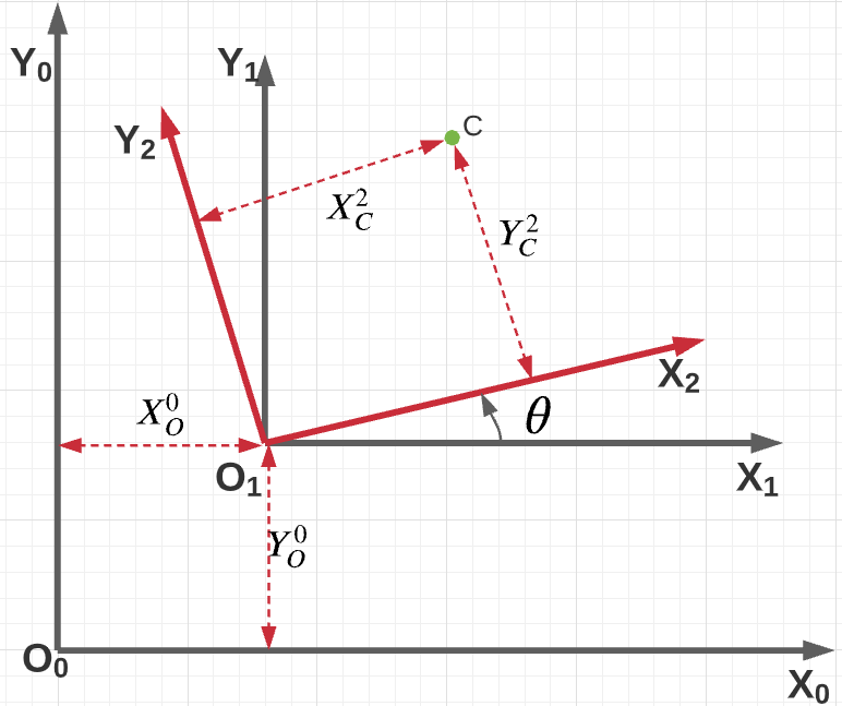
Assume a fixed frame $(O_0-X_0-Y_0)$ and a mobile frame $(O_1-X_1-Y_1)$. Let C be a point in space. The relation between both the frames and C can be derived using simple math.
The following equations can be written down based on the above figure
\[\hat{X_1} = (X_1\cos{\theta})\hat{X_0} + (X_1\sin{\theta})\hat{Y_0}\] \[\hat{Y_1} = - (Y_1\sin{\theta})\hat{X_0} + (Y_1\cos{\theta})\hat{Y_0}\]Upon rearranging the terms,
\[\begin{equation*} \begin{bmatrix} \hat{X_1}\\ \hat{Y_1}\\ \end{bmatrix} = \begin{bmatrix} \cos{\theta} & \sin{\theta}\\ -\sin{\theta} & \cos{\theta}\\ \end{bmatrix} \begin{bmatrix} \hat{X_0}\\ \hat{Y_0}\\ \end{bmatrix} \end{equation*}\]The above trigonometric matrix is called the rotation matrix, denoted by $R$. The relation between the coordinates of point C in the fixed and mobile frame can therefore be expressed as: \(C^1 = R_0^1C^0\)
Combined Translation & Rotation
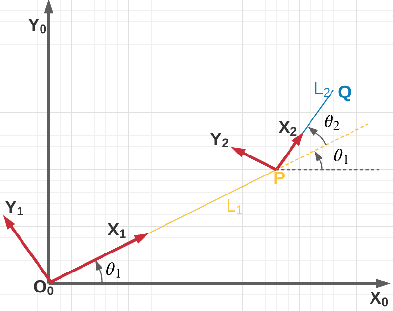
Assume a fixed frame $(O_0-X_0-Y_0)$ and a mobile frame $(O_2-X_2-Y_2)$. Let us assume an intermediate mobile frame given by $(O_1-X_1-Y_1)$. Let C be a point of interest, The frame $O_2$ can be generated by translation from frame $O_0$ to give frame $O_1$ and then rotation by $\theta$ to give frame $O_2$.
The coordinates of point C between the mobile and fixed frame can be related using the following:
\[C^0 = O_1^0 + R_1^0C^1\]2D - RR Manipulator
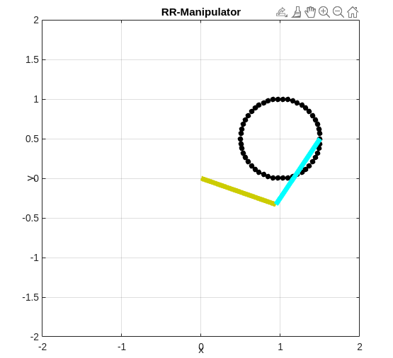
Consider the following manipulator diagram for a 2 DoF planar robotic arm.
$P^1 = \begin{bmatrix}
l_1
0
\end{bmatrix};$
$Q^2 = \begin{bmatrix}
l_2
0
\end{bmatrix};$
$P^0 = R_1^0P^1$
$Q^1 = R_2^1Q^2 + P^1$
$Q^0 = R_1^0Q^1 = R_1^0(R_2^1Q^2 + P^1)$
\[\begin{align} P^0 &= \begin{bmatrix} X_p^0\\ Y_p^0\\ \end{bmatrix}= \begin{bmatrix} l_1\cos{\theta_1}\\ l_1\sin{\theta_1} \end{bmatrix}\\ Q^0 &= \begin{bmatrix} X_Q^0\\ Y_Q^0\\ \end{bmatrix} = \begin{bmatrix} l_1\cos{\theta_1} + l_2\cos{(\theta_1+\theta_2)}\\ l_1\sin{\theta_1} + l_2\sin{(\theta_1+\theta_2)}\\ \end{bmatrix} \end{align}\]Forward Kinematics
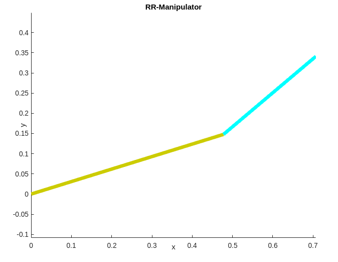
The equations for the RR manipulator can be used to draw the arm in MATLAB, the code for the same is given below.
1
2
3
4
5
6
7
8
9
10
11
12
13
14
15
16
17
18
19
20
21
22
23
24
25
26
27
%% Lec1_RRManu.m %%
clc
%clear all
close all
%% Manipulator Parameters
l1 = 0.5; l2 = 0.3;
theta1 = 0.3; theta2 = 0.4;

%% World Frame
x_0 = 0; y_0 = 0;

%% Link 1
x_p0 = l1 * cos(theta1);
y_p0 = l1 * sin(theta1);

%% Link 2
x_q0 = l1 * cos(theta1) + l2 * cos(theta1 + theta2);
y_q0 = l1 * sin(theta1) + l2 * sin(theta1 + theta2);

%% Draw Lines
line([x_0, x_p0], [y_0, y_p0], 'Linewidth', 5, 'Color', [204, 204, 1] / 255);
line([x_q0, x_p0], [y_q0, y_p0], 'Linewidth', 5, 'Color', 'cyan');
axis('equal');
xlabel('x');
ylabel('y');
title('RR-Manipulator')
Upon executing the code you should be able see something similar in your figure window.
Inverse Kinematics
We can also solve for $\theta_1$ and $\theta_2$ given the end-effector position. This is most useful in everyday life implementation as we often know one way or another to which position our arm should move. This approach is called inverse kinematics. Below given program is a simple example on how we can use matlab to solve the obtained system of non-linear equations for a given value of end-effector positions $\verb|x_ref,y_ref|$, using $fsolve$. Other numerical methods for solving system of non-linear equations that can be implemented from scratch will be discussed in later sections.
1
2
3
4
5
6
7
8
9
10
11
12
13
14
15
16
17
18
19
20
21
22
23
24
25
26
27
28
29
30
31
32
33
%% Lec2_InverseRRManu.m %%
clc
close all

l1 = 0.5; l2 = 0.5;
x_ref = 0.5; y_ref = 0;
param = [l1 l2 x_ref y_ref];

x0 = [0.1 0.1];
[x, fval, exitflag] = fsolve(@Lec2_InvFun, x0, optimoptions('fsolve', 'Display', 'iter'), param)

theta1 = x(1);
theta2 = x(2);

%% World Frame
x_0 = 0; y_0 = 0;

%% Link 1
x_p0 = l1 * cos(theta1);
y_p0 = l1 * sin(theta1);

%% Link 2
x_q0 = l1 * cos(theta1) + l2 * cos(theta1 + theta2);
y_q0 = l1 * sin(theta1) + l2 * sin(theta1 + theta2);

%% Draw Lines
line([x_0, x_p0], [y_0, y_p0], 'Linewidth', 5, 'Color', [204, 204, 1] / 255);
line([x_q0, x_p0], [y_q0, y_p0], 'Linewidth', 5, 'Color', 'cyan');
axis('equal');
xlabel('x');
ylabel('y');
title('RR-Manipulator')
As you might have noticed the above program depends on an external function called \verb|Lec2_InvFun|. The code for the function is given below.
1
2
3
4
5
6
7
8
9
10
11
12
13
14
15
16
%% Lec2_InvFun.m %%

function F = Lec2_InvFun(x, param)

l1 = param(1); l2 = param(2);
x_ref = param(3); y_ref = param(4);
theta1 = x(1); theta2 = x(2);

x_q0 = l1 * cos(theta1) + l2 * cos(theta1 + theta2);
y_q0 = l1 * sin(theta1) + l2 * sin(theta1 + theta2);

F = [x_q0 - x_ref; y_q0 - y_ref];

end
Upon executing the code you should be able see something similar in your figure window

Tracing Trajectories
If we can write the mathematical equation for a curve the x,y points on the curve can be passed into the inverse kinematics block for the manipulator which allows the robotic arm to trace the shape of the curve. The below given program does the same, it also shows the animation of the manipulator. Note, that the below given program uses $\verb|Lec2_InvFun|$ for running.
1
2
3
4
5
6
7
8
9
10
11
12
13
14
15
16
17
18
19
20
21
22
23
24
25
26
27
28
29
30
31
32
33
34
35
36
37
38
39
40
41
42
43
44
45
46
47
48
49
50
51
52
53
54
55
56
57
58
59
60
61
62
63
%% Lec2_TrajManu.m %%

clc
close all

%% Parameter Setting
l1 = 1; l2 = 1;

%% Trajectory Generator
phi = linspace(0, 2 * pi, 51);
x_ref = 1 + 0.5 * cos(phi); y_ref = 0.5 + 0.5 * sin(phi);

theta1 = 0.5; theta2 = 0.5;
theta1_f = zeros(length(phi), 1);
theta2_f = zeros(length(phi), 1);

for i = 1:length(phi)
    theta = [theta1, theta2];
    options = optimoptions('fsolve', 'Display', 'Off', 'MaxIter', 100, 'MaxFunEval', 300);
    param = [l1 l2 x_ref(i) y_ref(i)];
    [x, fval, exitflag] = fsolve(@Lec2_InvFun, theta, options, param);

    theta1 = x(1); theta2 = x(2);

    theta1_f(i, 1) = x(1);
    theta2_f(i, 1) = x(2);

end

%% World Frame
x_0 = 0; y_0 = 0;

%% Animation
for i = 1:length(phi)

    % Link 1
    x_p0 = l1 * cos(theta1_f(i));
    y_p0 = l1 * sin(theta1_f(i));

    % Link 2
    x_q0 = l1 * cos(theta1_f(i)) + l2 * cos(theta1_f(i) + theta2_f(i));
    y_q0 = l1 * sin(theta1_f(i)) + l2 * sin(theta1_f(i) + theta2_f(i));

    % Tracer
    plot(x_q0, y_q0, 'ko', "MarkerSize", 5, 'MarkerEdgeColor', 'k', 'MarkerFaceColor', 'k');
    hold on;

    h1 = line([x_0, x_p0], [y_0, y_p0], 'Linewidth', 5, 'Color', [204, 204, 1] / 255);
    h2 = line([x_q0, x_p0], [y_q0, y_p0], 'Linewidth', 5, 'Color', 'cyan');
    grid on;
    axis('equal');
    xlabel('x');
    ylabel('y');
    title('RR-Manipulator')
    xlim([- 2 2]);
    ylim([- 2 2]);

    pause(0.3);
    if i < length(phi)
        delete(h1);
        delete(h2);
    end
end
Upon executing the code you should be able see something similar in your figure window
Differential Drive
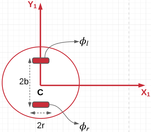
Consider a fixed frame ($O_0-X_0-Y_0$) and a mobile frame ($O_1-X_1-Y_1$), the mobile frame is attached to a two wheel differential drive robot, such that the $X_1$ axis is pointing forwards and the $Y_1$ is perpendicular to the orientation of the wheels.
Let $r$ be the radius of the wheels and $2b$ be the distance between the wheels, and $\theta$ be the angle the angle the mobile frame makes with the horizontal of the fixed frame.
Forward Kinematics
The forward kinematics of the differential drive car involves finding ($X_C^0(t),Y_C^0(t)$) given $b,r$, initial position ($X_C^0(t=0),Y_C^0(t=0)$) and the driving history of the robot ($\dot{\phi_r}(t),\dot{\phi_l}(t)$).
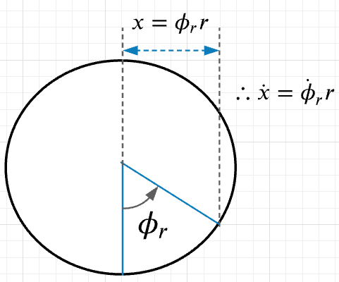
The distance traveled by the wheel if it rotates by an angle $\phi$ is given by $r\phi$. The rate of change of distance travelled by the wheel is therefore given by $r\dot{\phi}$. Assuming the right wheel is denoted by the subscript r, similar assumptions and derivations can be made for the left wheel.
Case 1: $\dot{\phi_l}=0, \dot{\phi_r}\neq0$
The distance moved by the right wheel is given by, $X_{wr}=r\phi_r$. The velocity of the right wheel is given by,
\[\dot{X_{wr}^1} =r\dot{\phi_r}\]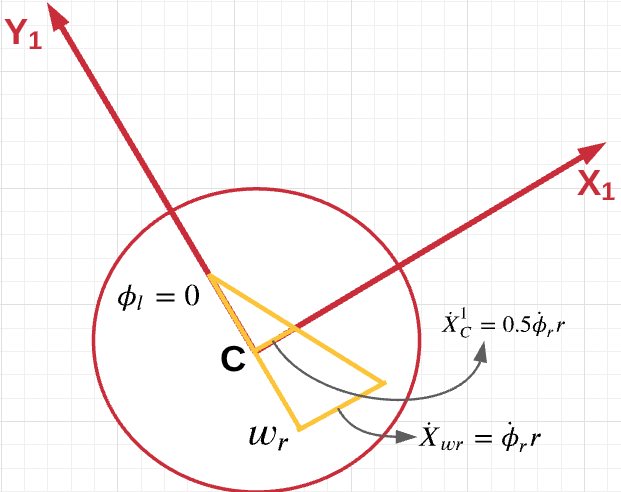
From geometry, the speed of the center C in the direction of $X_1$ can be written as,
\[\dot{X_C^1}= 0.5r\dot{\phi_r}\]Case 2: $\dot{\phi_l}\neq0, \dot{\phi_r}=0$
From symmetry similar arguments can be made for the left wheel, giving the following equations.
\[\dot{X_{wl}^1} =r\dot{\phi_l}\] \[\dot{X_C^1}= 0.5r\dot{\phi_l}\]From case 1 \& 2, the velocity of the point C in the directions of $X_1$ and $Y_1$ can be written down as,
\[\begin{align} \dot{X_C^1} &= 0.5r(\dot{\phi_l}+\dot{\phi_r})\\ \dot{Y_C^1} &= 0 \end{align}\]The velocity of point C in frame 0 and 1 can be related as,
\[\begin{align*} \dot{C^0} &= R_1^0\dot{C^1}\\ \begin{bmatrix} \dot{X_C^0}\\ \dot{Y_C^0} \end{bmatrix} &= \begin{bmatrix} \cos{\theta} & -\sin{\theta}\\ \sin{\theta} & \cos{\theta}\\ \end{bmatrix} \begin{bmatrix} \dot{X_C^1}\\ \dot{Y_C^1} \end{bmatrix}\\ \begin{bmatrix} \dot{X_C^0}\\ \dot{Y_C^0} \end{bmatrix} &= \begin{bmatrix} \cos{\theta} & -\sin{\theta}\\ \sin{\theta} & \cos{\theta}\\ \end{bmatrix} \begin{bmatrix} 0.5r(\dot{\phi_r}+\dot{\phi_l})\\ 0 \end{bmatrix}\\ \dot{X_C^0(t)} &= 0.5r(\dot{\phi_r}+\dot{\phi_l})\cos{\theta}\\ \dot{Y_C^0(t)} &= 0.5r(\dot{\phi_r}+\dot{\phi_l})\sin{\theta} \end{align*}\]For finding the expression for rate of change of $\theta$,
Case 1: $\dot{\phi_l}=0, \dot{\phi_r}\neq0$
\[X_{wr} = r\phi_r\]from geometry,
\[X_{wr} = 2b\theta\]therefore gives,
\[\dot{\theta} = \dfrac{r\dot{\phi_r}}{2b}\]Similar arguments can be made for the other case, only exception being the angle $\theta$ is negative. Therefore from case 1 and 2 the following can be derived.
\[\dot{\theta} = \dfrac{r}{2b}(\dot{\phi_r}-\dot{\phi_l})\]Therefore to summarize,
\[\begin{align*} \dot{X_C^0} &= v\cos{\theta}\\ \dot{Y_C^0} &= v\sin{\theta}\\ \dot{\theta} &= \omega\\ v &= 0.5r(\dot{\phi_r}+\dot{\phi_l})\\ w &= \dfrac{r}{2b}(\dot{\phi_r}-\dot{\phi_l}) \end{align*}\]To find $X_C^0,Y_C^0,\theta$, we will be using Euler’s integration.
\[\begin{align*} \dot{X_C^0} &= \dfrac{X_C(t_{i+1})-X_C(t_i)}{t_{i+1}-t_i} = v(t_i)\cos{\theta(t_i)}\\ \dot{Y_C^0} &= \dfrac{Y_C(t_{i+1})-Y_C(t_i)}{t_{i+1}-t_i} = v(t_i)\sin{\theta(t_i)}\\ \dot{\theta} &= \dfrac{\theta(t_{i+1})-\theta(t_i)}{t_{i+1}-t_i} = \omega(t_i) \end{align*}\]Upon rearranging the terms,
\[\begin{align*} X_C^0(t_{i+1}) &= X_C^0(t_{i}) + hv(t_{i})\cos{\theta(t_i)}\\ Y_C^0(t_{i+1}) &= Y_C^0(t_{i}) + hv(t_{i})\sin{\theta(t_i)}\\ \theta(t_{i+1}) &= \theta(t_i) + h\omega(t_i) \end{align*}\]1
2
3
4
5
6
7
8
9
10
11
12
13
14
15
16
17
18
19
20
21
22
23
24
25
26
27
28
29
30
31
32
33
34
35
36
37
38
39
40
41
42
43
44
45
46
47
48
49
50
51
52
53
54
55
56
%% Lec3_DiffCar.m %%
clc
close all
parms.R = 0.1; %Radius of the chassis for animation
% parms.writeMovie = 0; %set to 1 to get a movie output
% parms.nameMovie = 'car.avi';
%% Initialize States
fps = 10;
parms.delay = 0.2;
z0 = [0 0 - pi / 2]; %initial position of the car
h = 0.1; %step size
%% Motion
t1 = 0:h:1;
speed1 = ones(1, length(t1));
omega1 = zeros(1, length(t1));
t2 = 1 + h:h:2;
speed2 = zeros(1, length(t2));
omega2 = pi / 2 * ones(1, length(t2));
t3 = 2 + h:h:3;
speed3 = ones(1, length(t3));
omega3 = zeros(1, length(t3));
t4 = 3 + h:h:4;
t5 = 4 + h:h:5;
t6 = 5 + h:h:6;
t7 = 6 + h:h:7;
t = [t1 t2 t3 t4 t5 t6 t7];
speed = [speed1 speed2 speed3 speed2 speed3 speed2 speed3];
omega = [omega1 omega2 omega3 omega2 omega3 omega2 omega3];
%% Euler Integration
z = z0; %Initial parameters
for i = 1:length(t) - 1
u = [speed(i) omega(i)];
zz = Lec3_Euler(h, z0, u);
z0 = zz;
z = [z; z0];
end
% t_interp = linspace(0,t(end),fps*t(end));
% [m,n] = size(z);
% for i=1:n
% z_interp(:,i) = interp1(t,z(:,i),t_interp);
% end
%% Animation
figure(1)
Lec3_Animate(t, z, parms);
1
2
3
4
5
6
7
8
9
10
11
12
13
14
15
16
17
18
19
20
21
22
23
24
25
26
27
28
29
30
31
32
33
34
35
36
37
38
39
40
41
42
43
44
45
46
47
48
%% Lec3_Animate.m %%

function Lec3_Animate(t, z, parms)
R = parms.R;
phi = linspace(0, 2 * pi);
x_circle = R * cos(phi);
y_circle = R * sin(phi);

% if (parms.writeMovie)
%     mov = VideoWriter(parms.nameMovie);
%     open(mov);
%end

n = length(t);
for i = 1:n
    theta = z(i, 3);
    x_robot = z(i, 1) + x_circle;
    y_robot = z(i, 2) + y_circle;
    x_dir = z(i, 1) + [0 R * cos(theta)];
    y_dir = z(i, 2) + [0 R * sin(theta)];

    plot(z(1:i, 1), z(1:i, 2), 'r', 'Linewidth', 2); hold on;
    light_blue = [176, 224, 230] / 255;
    h1 = patch(x_robot, y_robot, light_blue);
    h2 = line(x_dir, y_dir, 'Color', 'black', 'Linewidth', 2);
    axis('equal');
    %span = max([-min(min(z(:,1:2))) max(max(z(:,1:2)))]);
    %span = max([span 2]);
    %axis([-span span -span span]);
    axis([- 2 2 - 2 2]);
    grid on;

    pause(parms.delay)
    delete(h1);
    delete(h2);
    %     if (parms.writeMovie)
    %         axis off %does not show axis
    %         set(gcf,'Color',[1,1,1]) %set background to white
    %         writeVideo(mov,getframe);
    %     end

end

% if (parms.writeMovie)
%     close(mov);
end
1
2
3
4
5
6
7
8
9
10
11
12
13
14
15
16
17
18
19
20
21
22
23
24
%% Lec3_Euler.m %%

function F = Lec3_Euler(h, z0, u)

v = u(1);
omega = u(2);

x_t0 = z0(1);
y_t0 = z0(2);
theta_t0 = z0(3);

xdot_c = v * cos(theta_t0);
ydot_c = v * sin(theta_t0);
thetadot = omega;

x_t1 = x_t0 + xdot_c * h;
y_t1 = y_t0 + ydot_c * h;
theta_t1 = theta_t0 + thetadot * h;

F = [x_t1, y_t1, theta_t1];

end
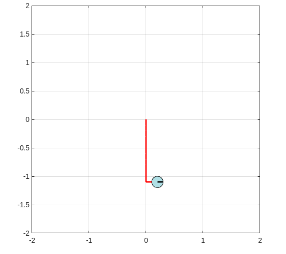
Upon successful execution of the above program you should be able to see a figure similar to this
Inverse Kinematics
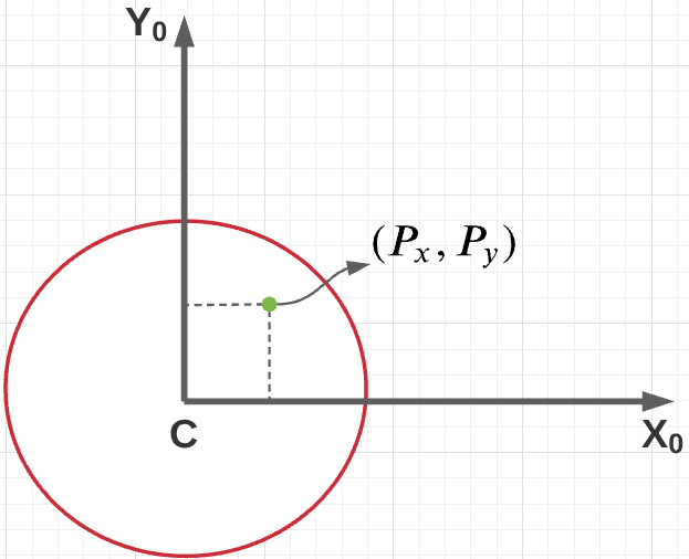
Inverse Kinematics is defined as finding the values of $v,\omega$ given ($X_P^0,Y_p^0$) as a function of time, where $P$ is a point fixed on the robot as shown in the figure.
From previous sections, we have the following relations
\[\begin{align*} P^0 &= R_1^0P^1\\ C^0 &= R_1^0C^1\\ P^0 - C^0 &= R_1^0(P^1-C^1)\\ \begin{bmatrix} X_P^0 - X_C^0\\ X_P^0 - Y_C^0 \end{bmatrix} &= \begin{bmatrix} \cos{\theta} & -\sin{\theta}\\ \sin{\theta} & \cos{\theta} \end{bmatrix} \begin{bmatrix} X_P^1 - X_C^1\\ Y_p^1 - Y_C^1 \end{bmatrix}\\ \begin{bmatrix} X_P^0 - X_C^0\\ X_P^0 - Y_C^0 \end{bmatrix} &= \begin{bmatrix} \cos{\theta} & -\sin{\theta}\\ \sin{\theta} & \cos{\theta} \end{bmatrix} \begin{bmatrix} P_X\\ P_Y \end{bmatrix}\\ \begin{bmatrix} X_P^0\\ Y_P^0 \end{bmatrix} &= \begin{bmatrix} X_C^0\\ Y_C^0 \end{bmatrix} + \begin{bmatrix} \cos{\theta} & -\sin{\theta}\\ \sin{\theta} & \cos{\theta} \end{bmatrix} \begin{bmatrix} P_X\\ P_Y \end{bmatrix}\\ \begin{bmatrix} X_C^0\\ Y_C^0 \end{bmatrix} &= \begin{bmatrix} X_P^0\\ Y_P^0 \end{bmatrix} + \begin{bmatrix} \cos{\theta} & -\sin{\theta}\\ \sin{\theta} & \cos{\theta} \end{bmatrix} \begin{bmatrix} P_X\\ P_Y \end{bmatrix}\\ \end{align*}\]Differentiating the above equations with time,
\[\begin{align*} \begin{bmatrix} \dot{X_P^0}\\ \dot{Y_P^0} \end{bmatrix} &= \begin{bmatrix} \dot{X_C^0}\\ \dot{Y_C^0} \end{bmatrix} + \begin{bmatrix} \dot{\theta}\sin{\theta} & -\dot{\theta}\cos{\theta}\\ \dot{\theta}\cos{\theta} & -\dot{\theta}\sin{\theta} \end{bmatrix} \begin{bmatrix} P_X\\ P_Y \end{bmatrix}\\ \begin{bmatrix} \dot{X_P^0}\\ \dot{Y_P^0} \end{bmatrix} &= \begin{bmatrix} v\cos{\theta}\\ v\sin{\theta} \end{bmatrix} + \begin{bmatrix} \omega\sin{\theta} & -\omega\cos{\theta}\\ \omega\cos{\theta} & -\omega\sin{\theta} \end{bmatrix} \begin{bmatrix} P_X\\ P_Y \end{bmatrix}\\ \begin{bmatrix} \dot{X_P^0}\\ \dot{Y_P^0} \end{bmatrix} &= \begin{bmatrix} \cos{\theta} & (-P_X\sin{\theta} - P_Y\cos{\theta})\\ \sin{\theta} & (P_X\cos{\theta} - P_Y\sin{\theta}) \end{bmatrix} \begin{bmatrix} v\\ \omega \end{bmatrix} \end{align*}\]We will be using a proportional controller for driving the error towards zero.
\[\dot{X_P^0} = K_{P_x}(X_{ref}-X_P^0)\] \[\dot{Y_P^0} = K_{P_Y}(Y_{ref}-Y_P^0)\]Where $K_{P_x},K_{P_y}$ are user chosen gains and $X_{ref},Y_{ref}$ are the desired reference points. Substituting these values in the above derived equations. \(\begin{align*} \begin{bmatrix} K_{P_x}(X_{ref}-X_P^0)\\ K_{P_Y}(Y_{ref}-Y_P^0) \end{bmatrix} &= \begin{bmatrix} \cos{\theta} & (-P_X\sin{\theta} - P_Y\cos{\theta})\\ \sin{\theta} & (P_X\cos{\theta} - P_Y\sin{\theta}) \end{bmatrix} \begin{bmatrix} v\\ \omega \end{bmatrix}\\ \begin{bmatrix} v\\ \omega \end{bmatrix} &= \begin{bmatrix} \cos{\theta} - \left(\dfrac{P_X}{P_Y}\right) \sin{\theta} & \sin{\theta} + \left( \dfrac{P_X}{P_Y}\right) \cos{\theta}\\ -\left( \dfrac{1}{P_X}\right) \sin{\theta} & -\left( \dfrac{1}{P_X}\right) \cos{\theta} \end{bmatrix} \begin{bmatrix} K_{P_x}(X_{ref}-X_P^0)\\ K_{P_Y}(Y_{ref}-Y_P^0) \end{bmatrix} \end{align*}\)
Also from forward kinematics we know the following,
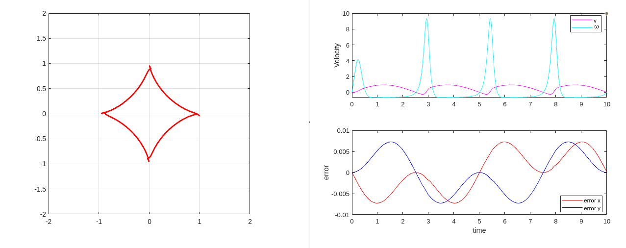
\[\begin{align*} \dot{X_C^0} &= v\cos{\theta}\\ \dot{Y_C^0} &= v\sin{\theta}\\ \dot{\theta} &= \omega \end{align*}\]All of the above derived equations can be used to create a trajectory following differential drive robot the code attached below follows a mathematical trajectory called “astroid” the code also has an PD controller implemented to keep the error close to zero.
1
2
3
4
5
6
7
8
9
10
11
12
13
14
15
16
17
18
19
20
21
22
23
24
25
26
27
28
29
30
31
32
33
34
35
36
37
38
39
40
41
42
43
44
45
46
47
48
49
50
51
52
53
54
55
56
57
58
59
60
61
62
63
64
65
66
67
68
69
70
71
%% Lec4_InvDiff.m %%

clc
close all
%% Parameters
parms.R = 0.1;
parms.px = 0.05;
parms.py = 0;
parms.Kp = 100;
parms.Kd = 0.5;
parms.delay = 0.001;
t0 = 0;
tend = 10;
fps = 10;
t = t0:0.01:tend;
h = 0.01;
%% Trajectory
x_center = 0;
y_center = 0;
a = 1;
x_ref = x_center + a * cos(2 * pi * t / tend) .^ 3;
y_ref = y_center + a * sin(2 * pi * t / tend) .^ 3;
%% Initilization
theta0 = pi / 2;
[x0 y0] = Lec4_ptP_to_ptC(x_ref(1), y_ref(1), theta0, parms);
z0 = [x0 y0 theta0];
z = z0;
e = [0 0];
v = 0;
omega = 0;
for i = 1:length(t) - 1
    x_c = z(end, 1);
    y_c = z(end, 2);
    theta = z(end, 3);

    [x_p, y_p] = Lec4_ptC_to_ptP(x_c, y_c, theta, parms);

    error = [x_ref(i + 1) - x_p y_ref(i + 1) - y_p];
    e = [e; error];
    err_p_dot = [parms.Kp * error(1) + parms.Kd * ((e(end, 1) - e(end - 1, 1)) / h); parms.Kp * error(2) + parms.Kd * ((e(end, 2) - e(end - 1, 2)) / h)];
    c = cos(theta); s = sin(theta);
    px = parms.px; py = parms.py;
    A = [c - (py / px) * s s + (py / px) * c; ...
     - (1 / px) * s (1 / px) * c];
    u = A * err_p_dot; %u = [v omega]
    v = [v; u(1)];
    omega = [omega; u(2)];
    %zz = ode4(@Lec4_RHS,[t(i) t(i+1)],z0,u);
    zz = Lec3_Euler(h, z0, u);
    z0 = zz(end, :);
    z = [z; z0];
end
t_interp = linspace(t0, tend, fps * tend);
[m, n] = size(z);
for i = 1:n
    z_interp(:, i) = interp1(t, z(:, i), t_interp);
end
figure(1)
Lec3_Animate(t_interp, z_interp, parms);
figure(2)
subplot(2, 1, 1)
plot(t, v, 'm'); hold on
plot(t, omega, 'c');
ylabel('Velocity');
legend('v', '\omega', 'Location', 'Best');
subplot(2, 1, 2)
plot(t, e(:, 1), 'r'); hold on
plot(t, e(:, 2), 'b');
legend('error x', 'error y', 'Location', 'Best');
ylabel('error');
xlabel('time');
1
2
3
4
5
6
7
8
9
%% Lec4_ptC_to_ptP.m %%

function [x_p, y_p] = Lec4_ptC_to_ptP(x_c, y_c, theta, parms)
c = cos(theta); s = sin(theta);
p = [parms.px; parms.py];
Xp = [c - s; s c] * p + [x_c; y_c];
x_p = Xp(1); y_p = Xp(2);

end
1
2
3
4
5
6
7
8
%% Lec4_ptP_to_ptC.m %%
function [x_c, y_c] = Lec4_ptP_to_ptC(x_p, y_p, theta, parms)
c = cos(theta); s = sin(theta);
p = [parms.px; parms.py];
Xc = - [c - s; s c] * p + [x_p; y_p];
x_c = Xc(1); y_c = Xc(2);

end
1
2
3
4
5
6
7
8
9
10
11
12
13
14
15
16
17
18
19
20
21
22
23
24
25
26
27
28
29
30
31
32
33
34
35
36
37
38
39
40
41
42
43
44
45
46
47
48
49
50
51
52
53
54
55
56
57
58
59
60
61
62
63
64
65
66
67
68
%% ode4.m %%

function Y = ode4(odefun, tspan, y0, varargin)
%ODE4  Solve differential equations with a non-adaptive method of order 4.
%   Y = ODE4(ODEFUN,TSPAN,Y0) with TSPAN = [T1, T2, T3, ... TN] integrates
%   the system of differential equations y' = f(t,y) by stepping from T0 to
%   T1 to TN. Function ODEFUN(T,Y) must return f(t,y) in a column vector.
%   The vector Y0 is the initial conditions at T0. Each row in the solution
%   array Y corresponds to a time specified in TSPAN.
%
%   Y = ODE4(ODEFUN,TSPAN,Y0,P1,P2...) passes the additional parameters
%   P1,P2... to the derivative function as ODEFUN(T,Y,P1,P2...).
%
%   This is a non-adaptive solver. The step sequence is determined by TSPAN
%   but the derivative function ODEFUN is evaluated multiple times per step.
%   The solver implements the classical Runge-Kutta method of order 4.
%
%   Example
%         tspan = 0:0.1:20;
%         y = ode4(@vdp1,tspan,[2 0]);
%         plot(tspan,y(:,1));
%     solves the system y' = vdp1(t,y) with a constant step size of 0.1,
%     and plots the first component of the solution.
%

if ~ isnumeric(tspan)
    error('TSPAN should be a vector of integration steps.');
end

if ~ isnumeric(y0)
    error('Y0 should be a vector of initial conditions.');
end

h = diff(tspan);
if any(sign(h(1)) * h <= 0)
    error('Entries of TSPAN are not in order.')
end

try
    f0 = feval(odefun, tspan(1), y0, varargin{:});
catch
    msg = ['Unable to evaluate the ODEFUN at t0,y0. ', lasterr];
    error(msg);
end

y0 = y0(:); % Make a column vector.
if ~ isequal(size(y0), size(f0))
    error('Inconsistent sizes of Y0 and f(t0,y0).');
end

neq = length(y0);
N = length(tspan);
Y = zeros(neq, N);
F = zeros(neq, 4);

Y(:, 1) = y0;
for i = 2:N
    ti = tspan(i - 1);
    hi = h(i - 1);
    yi = Y(:, i - 1);
    F(:, 1) = feval(odefun, ti, yi, varargin{:});
    F(:, 2) = feval(odefun, ti + 0.5 * hi, yi + 0.5 * hi * F(:, 1), varargin{:});
    F(:, 3) = feval(odefun, ti + 0.5 * hi, yi + 0.5 * hi * F(:, 2), varargin{:});
    F(:, 4) = feval(odefun, tspan(i), yi + hi * F(:, 3), varargin{:});
    Y(:, i) = yi + (hi / 6) * (F(:, 1) + 2 * F(:, 2) + 2 * F(:, 3) + F(:, 4));
end
Y = Y.';
1
2
3
4
5
6
7
8
9
10
%% Lec4_RHS.m %%

function zdot = Lec4_RHS(t, z, u)
v = u(1); omega = u(2);
theta = z(3);
x_c_dot = v * cos(theta);
y_c_dot = v * sin(theta);
theta_dot = omega;
zdot = [x_c_dot y_c_dot theta_dot]';
Upon successful execution of the above program, you will end up with the following two figures.
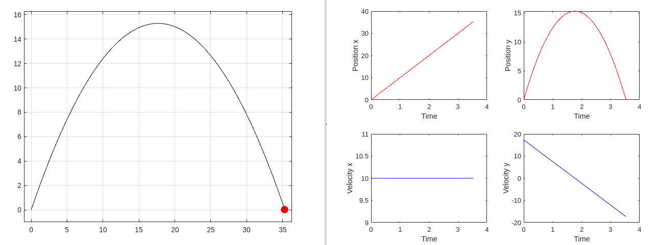
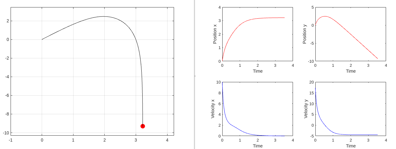
Projectile Motion
2-D projectile motion will be analyzed in this section, Euler Lagrange Equations will be introduced and used for finding out the equations of motion of the projectile.
Forward Kinematics
Let the position of the projectile wrt to the fixed frame be denoted as ($X,Y$). The launch angle is denoted by $\theta$ and the drag force is given by $\vec{F_d}=-Cv^2\hat{v}$.
\[\vec{F_d}=-Cv^2\hat{v} = -Cv^2\dfrac{\vec{v}}{|\vec{v}|} = -C|v|\hat{v}\] \[F_x = -C\dot{x}\sqrt{\dot{x}^2 + \dot{y}^2}\] \[F_y = -C\dot{y}\sqrt{\dot{x}^2 + \dot{y}^2}\]From Euler-Lagrange Formulaizm,
\[\begin{align*} L &= T - V\\ T &= 0.5mv^2 = 0.5m(\dot{x}^2+\dot{y}^2)\\ V &= mgy\\ L &= 0.5m(\dot{x}^2+\dot{y}^2) - mgy \end{align*}\]Given that,
\[\begin{align*} \dfrac{d}{dt}\left(\dfrac{\partial L}{\partial \dot{q_j}}\right) - \dfrac{\partial L}{\partial q_j} &= Q_j \end{align*}\]In the direction of x,
\[\begin{align*} \dfrac{d}{dt}\left(\dfrac{\partial (0.5m(\dot{x}^2+\dot{y}^2 )-mgy)}{\partial \dot{x}}\right) - \dfrac{\partial (0.5m(\dot{x}^2+\dot{y}^2 )-mgy)}{\partial x} &= -C\dot{x}\sqrt{\dot{x}^2+\dot{y}^2}\\ \ddot{x} &= -\dfrac{C}{m}\dot{x}\sqrt{\dot{x}^2+\dot{y}^2} \end{align*}\]In the direction of y,
\[\begin{align*} \dfrac{d}{dt}\left(\dfrac{\partial (0.5m(\dot{x}^2+\dot{y}^2 )-mgy)}{\partial \dot{y}}\right) - \dfrac{\partial (0.5m(\dot{x}^2+\dot{y}^2 )-mgy)}{\partial y} &= -C\dot{y}\sqrt{\dot{x}^2+\dot{y}^2}\\ \ddot{y} &= -g -\dfrac{C}{m}\dot{y}\sqrt{\dot{x}^2+\dot{y}^2} \end{align*}\]Integrating $\ddot{x}$ and $\ddot{y}$ $\textit{wrt}$ time should give us $\dot{x},\dot{y},x,y$.